"Talk is cheap. Show me the code."
— Linus Torvalds, popularised in the film The Social Network (2010)
The previous chapter laid out the what and the why of the
quantitative toolkit. This chapter is the how — the Python
foundations that turn the equations of Chapter 2 into pipelines you
can actually run, refit, and ship. We start with data processing
using Polars DataFrames, then move to visualization for exploratory
analysis and model interpretation. Finally, we cover the transition
to NumPy arrays and PyTorch tensors for machine learning, along with
time-series libraries that streamline forecasting workflows.
The progression follows a natural workflow: process data
(Section 03-01) → visualize patterns (Section 03-02) → convert
to arrays/tensors (Section 03-03) → use specialized libraries
(Sections 03-04 and 03-05).
Contents
DataFrames with Polars — efficient data
processing with expression-based operations, time-series patterns,
and lazy evaluation.
Time-Series Forecasting with sktime —
splitters, evaluators, and the unified forecasting interface that
makes Chapter 4's baselines portable.
DataFrames with Polars
DataFrames are the cornerstone of financial data analysis. Whether you're building forecasting models, computing risk metrics, or preparing features for machine learning, you'll spend most of your time manipulating tabular data. This chapter introduces Polars—a DataFrame library designed for the scale and complexity of modern financial AI systems.
Why Polars for Finance AI?
Financial data presents unique challenges: you work with cross-asset panels spanning thousands of tickers, time-series operations that must respect calendar boundaries, and sparse event data (earnings, dividends, corporate actions) that must align precisely with price data. Traditional DataFrame libraries struggle with these patterns, forcing you to write slow loops or drop into low-level code.
Polars solves this by combining familiar DataFrame ergonomics with an Apache Arrow memory layout, vectorized expressions, multi-threaded execution, and a query optimizer that fuses operations into efficient pipelines. As a result, You can handle large cross-asset panels, compute rolling statistics across thousands of time series, and join sparse events to dense price data—all without writing bespoke C++ or sacrificing code readability.
Learning Polars as a Pattern Language
Rather than treating Polars as just another DataFrame library, we'll approach it as a pattern language for financial workflows. Each example in this section introduces reusable idioms that solve common finance problems:
Per-ticker operations: Computing returns, rolling statistics, and lags for each asset independently
Calendar-aware resampling: Aggregating daily data to monthly or quarterly buckets while respecting trading calendars
Sparse event joins: Aligning dividends, earnings, and other events with price data without look-ahead bias
Lazy pipeline templates: Building efficient feature engineering pipelines that scale to large datasets
These patterns appear throughout the book—in forecasting models (Chapter 4), factor construction and dynamic modeling (Chapter 6), and agent workflows (Chapter 8).
Expressions
One of the key features in Polars is expression-based execution. Traditional pandas DataFrames use an imperative pattern where you modify the DataFrame step-by-step. Polars uses a declarative, expression-based approach that feels like writing SQL queries.
Pandas (Imperative Pattern):
import pandas as pd# Each operation modifies the DataFrame in placedf['Return'] = df['Close'] / df['Close'].shift(1) - 1df['ReturnZ'] = (df['Return'] - df['Return'].mean()) / df['Return'].std()df = df[df['Volume'] > 1000000] # Filter modifies DataFrame
Polars (Expression-Based Pattern):
import polars as pl# All operations are expressions that compose togetherdf = df.with_columns([ ((pl.col("Close") / pl.col("Close").shift(1)) - 1).alias("Return"), ((pl.col("Return") - pl.col("Return").mean()) / pl.col("Return").std()).alias("ReturnZ")]).filter(pl.col("Volume") > 1_000_000)
Why Expressions Are SQL-Friendly and Beneficial:
Query Optimization: Polars can see your entire pipeline before execution, enabling optimizations like predicate pushdown, projection pruning, and operator fusion. The query optimizer rearranges operations for efficiency.
Readability: Expressions read like mathematical formulas or SQL queries, making complex transformations easier to understand and maintain.
Composability: Expressions can be combined, reused, and nested without side effects. You can build complex pipelines from simple building blocks.
Lazy Evaluation: Combined with .lazy(), expressions enable deferred execution where Polars optimizes the entire query before running it—critical for large financial datasets.
String Operations with .str Accessor:
Polars provides a .str accessor for string operations, similar to pandas but optimized:
# String operations on ticker symbolsdf = df.with_columns([ pl.col("Ticker").str.to_uppercase().alias("TickerUpper"), pl.col("Ticker").str.slice(0, 3).alias("TickerPrefix"), pl.col("Ticker").str.contains("ETF").alias("IsETF"), pl.col("Ticker").str.replace(" ", "-").alias("TickerNormalized"),])# Extract patterns (e.g., extract exchange from ticker format "AAPL:NASDAQ")df = df.with_columns([ pl.col("Ticker").str.split(":").list.get(1).alias("Exchange")])
Finance Use Case: Expression-based execution is especially powerful for financial workflows because:
Feature engineering often involves many chained transformations (returns → rolling stats → normalization)
Lazy evaluation lets you build entire pipelines that only execute when needed, reducing memory usage
Query optimization automatically handles common patterns like "filter early, select late" for better performance
Time Processing
Another unique characteristic of Polars is its powerful time-series processing capabilities. Financial data is inherently temporal, and Polars provides specialized functions for calendar-aware operations, rolling windows, date extraction, and time-based joins—all critical for avoiding look-ahead bias and respecting trading calendars.
1. group_by_dynamic: Calendar-Aware Grouping
Unlike fixed-window operations, group_by_dynamic respects actual calendar boundaries (months, quarters, weeks), which is essential for aligning with reporting periods and trading calendars.
Why this matters: Calendar months have different numbers of trading days. Fixed windows (e.g., "30 days") would misalign with reporting periods. group_by_dynamic ensures your aggregations align with actual calendar boundaries.
2. rolling: Fixed-Window Statistics
Rolling windows compute statistics over a fixed number of periods, essential for technical indicators and short-term features.
# Rolling statistics per tickerfeatures = prices.with_columns([ # 20-day moving average pl.col("Close").rolling_mean(20).over("Ticker").alias("MA20"), # 20-day rolling volatility pl.col("Return").rolling_std(20).over("Ticker").alias("Vol20"), # 10-day rolling high (for breakout detection) pl.col("Close").rolling_max(10).over("Ticker").alias("High10"),])
Finance use case: Volatility targeting, momentum signals, and technical indicators all rely on rolling windows. The .over("Ticker") ensures each asset's time series is processed independently.
Note: The first 9 rows show null for rolling statistics because a 10-period window requires at least 10 previous values. This is expected behavior—rolling windows need sufficient history before producing values.
3. dt Accessor: Date/Time Extraction
Extract calendar components for grouping, filtering, and feature engineering. This requires datasets with actual Date columns (like prices_daily.csv):
# Load data with Date column (e.g., prices_daily.csv)prices = pl.read_csv("data/prices_daily.csv", try_parse_dates=True)# Extract calendar componentsprices = prices.with_columns([ pl.col("Date").dt.year().alias("Year"), pl.col("Date").dt.quarter().alias("Quarter"), pl.col("Date").dt.month().alias("Month"), pl.col("Date").dt.weekday().alias("Weekday"), # 1=Monday, 7=Sunday pl.col("Date").dt.strftime("%Y-%m").alias("YearMonth"),])# Filter by fiscal periodsq4_data = prices.filter(pl.col("Date").dt.quarter() == 4)
Finance use case: Calendar effects (month-end, quarter-end patterns), fiscal period alignment, and seasonal feature engineering.
Filtering by date ranges: Use explicit date objects to stay calendar-aware. Unlike integer indexing, this respects actual calendar boundaries. This requires datasets with actual Date columns:
from polars import date# Load data with Date column (e.g., prices_daily.csv)prices = pl.read_csv("data/prices_daily.csv", try_parse_dates=True)# Filter recent data (e.g., for backtesting recent models)recent = prices.filter(pl.col("Date") >= date(2020, 1, 1))# Filter a specific historical period (e.g., a market cycle)past_cycle = prices.filter( pl.col("Date").is_between(date(2018, 1, 1), date(2020, 12, 31)))
Why calendar-aware matters: Financial contracts, reporting periods, and trading calendars depend on actual dates, not row counts. Using explicit dates prevents bugs when data has gaps (holidays, weekends, delistings).
4. join_asof: Time-Based Joins Without Look-Ahead Bias
Align sparse events (earnings, dividends) with price data using the most recent event available at each point in time—critical for avoiding look-ahead bias. This requires datasets with actual Date columns:
# Load data with Date columnsprices = pl.read_csv("data/prices_daily.csv", try_parse_dates=True)earnings = pl.read_csv("data/earnings.csv", try_parse_dates=True)# Join earnings announcements to prices (only use info available at that time)prices_with_earnings = ( prices.sort("Date") .join_asof( earnings.sort("AnnouncementDate"), left_on="Date", right_on="AnnouncementDate", by="Ticker", strategy="backward", # Use most recent earnings before/on this date tolerance=pl.duration(days=30), # Only match within 30 days ))
Why strategy="backward" matters: This ensures you only use events that occurred on or before the trading date. Using strategy="forward" would be look-ahead bias—using future information in your model.
Finance use case: Aligning earnings announcements, analyst upgrades, corporate actions, and other events with price data while maintaining temporal integrity.
Combining Time Operations:
These operations often work together in financial workflows:
# Build monthly features with rolling statisticsmonthly_features = ( prices.sort(["Ticker", "Date"]) .with_columns([ # Rolling features pl.col("Return").rolling_mean(20).over("Ticker").alias("MA20"), pl.col("Return").rolling_std(20).over("Ticker").alias("Vol20"), # Calendar features pl.col("Date").dt.quarter().alias("Quarter"), ]) .group_by_dynamic("Date", every="1mo", group_by="Ticker") .agg([ pl.col("MA20").last().alias("MonthMA20"), pl.col("Vol20").mean().alias("MonthVol20"), ]))
These time-series operations appear throughout the book—in forecasting models (Chapter 4), backtesting workflows, and factor construction (Chapter 6).
Schema Setup
You can start by installing Polars package using your preferred package manager:
pip install polars# oruv add polars
All examples in this book use a consistent set of CSV files that represent typical financial data you'll encounter in real workflows. Understanding this structure helps you see how Polars patterns apply to your own data.
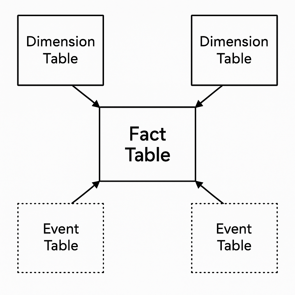
We organize the data using a star schema—a common pattern in financial data warehouses. Since this is not a book about database architecture, we will not dive deep into schema design. However, you need to be aware that financial data warehouses share a common data architecture pattern. The center consists of fact tables (dense, regularly updated data like prices, volumes), surrounded by dimension tables (metadata that changes slowly) and event tables (sparse, irregular occurrences).
Here's what each dataset represents:
dataset
contents (abridged)
role
when you'll use it
prices_daily.csv
tidy OHLCV + ticker identifiers for large-cap stocks/ETFs
Total return calculations, dividend yield features
options.csv
option chain quotes with strikes, expiries, Greeks
event
Volatility surface modeling, hedging strategies
analyst_recommendations.csv
upgrades/downgrades and target changes
event
Sentiment features, recommendation signals
ownership.csv
institutional holders and positions
cross-sectional
Ownership concentration factors
insider_transactions.csv
officer/director trades with roles, amounts, and cash value
event
Insider trading signals, corporate governance features
finance.csv
sample daily finance data from kaggle competition
overall
sample data for this section.
The star schema separates concerns cleanly. Dense fact tables (prices, fundamentals) are optimized for time-series operations. Sparse event tables (dividends, earnings) are joined in only when needed, avoiding memory bloat. Dimension tables (company info) provide stable metadata for cross-sectional analysis.
Why Star Schema for Finance AI:
Separation of Concerns:
Fact tables (prices, fundamentals) = Data that changes over time, optimized for time-series operations
Dimension tables (company info) = Metadata that changes slowly, provides stable reference data
Event tables (dividends, earnings) = Sparse, irregular occurrences that are joined only when needed
Memory Efficiency:
Load only what you need: start with fact tables (prices), join dimensions and events only when required
Example: Load price data first, then join dividend information only for total return calculations
Avoids loading entire event history into memory when you only need recent events
Query Performance:
Fact tables are optimized for time-series operations (rolling, grouping by date)
Dimension tables enable fast lookups for cross-sectional analysis
Event tables can be filtered before joining (e.g., only recent dividends)
Flexibility:
Build different feature sets by joining different combinations of tables
Easy to add new data sources without restructuring existing tables
Practical Example: Building a Feature Set
# Step 1: Load fact table (prices) - your core dataprices = pl.read_csv("data/prices_daily.csv", try_parse_dates=True)# Step 2: Join dimension table (company info) for cross-sectional featurescompany_info = pl.read_csv("data/company_info.csv")prices_with_metadata = prices.join(company_info, on="Ticker", how="left")# Step 3: Join event table (dividends) only when needed for total returnsdividends = ( pl.read_csv("data/corporate_actions.csv", try_parse_dates=True) .filter(pl.col("ActionType") == "dividend") .select(["Date", "Ticker", "Value"]) .rename({"Value": "Dividend"}))# Join events with time-aware join (no look-ahead bias)features = ( prices_with_metadata .join_asof( dividends.sort("Date"), left_on="Date", right_on="Date", by="Ticker", strategy="backward" ) .with_columns(pl.col("Dividend").fill_null(0.0)) .with_columns([ # Total return = price return + dividend yield (pl.col("Return") + pl.col("Dividend") / pl.col("Close")).alias("TotalReturn") ]))
Workflow Pattern:
Start with fact tables (prices) - this is your core time-series data
Join dimensions (company info) - for cross-sectional features and filtering
Join events (dividends, earnings) - for event-driven features, using time-aware joins
Build final feature matrix - combine all information for ML models
After all, in financial AI systems, all we need to know are "What will price be" and "How much to buy". The star schema is the best design for this because it separates the core time-series data (fact tables) from supporting information (dimensions and events). All the edge tables (dimensions, events) are just for providing useful information to build the final dataframe(s) that will inform the system's predictions and decisions.
This pattern appears throughout the book—when building forecasting features (Chapter 4), constructing factors (Chapter 6), and preparing data for AI agents (Chapter 8).
Explanatory Data Analysis with Polars
Let's start with exploring the data using Polars. In finance, it is always important to inspect your data before anything. Not only do data quality issues cause subtle bugs, but you also need to find meaningful patterns with intuition in order to do proper forecasting and dynamic modeling.
Why EDA Matters in Finance:
Data Quality Issues:
Missing prices, incorrect dates, or invalid values can break return calculations
Example: A single bad price can corrupt an entire backtest, leading to incorrect trading signals
Schema validation and sanity checks catch these issues early
Pattern Discovery:
Market regimes: Identify bull/bear markets, volatility regimes, and structural breaks
Volatility clustering: High volatility periods followed by high volatility (GARCH effects)
Cross-asset relationships: Correlations that change over time, factor exposures
AI Limitations and Human Guidance:
One common misconception about artificial intelligence in finance is that AI will solve everything. That's not true.
AI has the capability of processing vast amounts of information, but it is the human's job to guide it to make the right decision.
In fact, because finance and economics mostly face data scarcity issues (limited historical data, regime changes), relying solely on deep learning or AI agents is likely to cause more harm than good.
EDA helps you understand what patterns exist, what assumptions are reasonable, and when models might break
Validation of Assumptions:
Statistical models assume certain distributions (e.g., returns are normally distributed)
EDA reveals when assumptions are violated (fat tails, skewness, non-stationarity)
This informs model choice: use robust methods when assumptions fail
Data Quality Checklist:
Before building models, validate your data:
Schema validation: Expected columns and types match actual data
Price bounds: Prices should be positive and within reasonable ranges
OHLC relationships: High >= Low, High >= max(Open, Close), Low <= min(Open, Close)
Volume: Non-negative, and zero volume should only occur on non-trading days
Returns: Daily returns typically within -50% to +50% (adjust for asset class)
Date ranges: Dates should be within expected historical range
Missing data patterns: Concentrated (one ticker) vs. widespread (all tickers on same dates)
Temporal ordering: No future data leakage (dates should be sorted, no look-ahead)
Connection to Visualization:
EDA is closely tied to visualization (Section 2). Visual inspection helps identify:
Relationships between variables (correlations, scatter plots)
We'll cover visualization patterns in Section 2 that complement the Polars operations shown here.
In terms of polars and csv, a csv file might have dates as strings, volumes as nullable integers, or missing values represented as empty strings. Polars doesn't carry an implicit index like pandas, so every join, filter, or resample must reference explicit columns—making schema validation critical.
finance.csv data
Let's start with simple explanatory analysis with finance.csv data from kaggle competition for daily market prediction portfolio optimization. We start with this data because it is simplest, preprocessed, frequency synchronized data which is easy for us to dive into polars dataframe. You can run head, describe methods to check the basic data structure.
import polars as pldf = pl.read_csv("./data/finance.csv")print(df.head())print(df.describe())
Missing values: Many columns have significant sparsity (e.g., E7: 77% missing, V10: 67% missing)
As you can see from the result, despite the fact that data is already processed, there are lots of NaN values. This is one of the crucial issues in financial data since data frequencies differ and observed times differ. For example:
Different frequencies: Some features might be computed daily, others weekly or monthly
Market holidays: Create gaps in time series (no trading data on weekends/holidays)
Corporate actions: Stock splits, delistings create missing periods
Data source timing: Different data providers update at different times
We will deal with this throughout this book with various strategies:
Forward-fill: For slowly-changing variables (e.g., fundamentals within a quarter)
Zero-fill: For missing returns (assuming no price change)
Drop rows: For extended gaps (e.g., delisted stocks)
Missing indicators: Add features that flag when data is imputed
The key is to handle missing data in a way that doesn't introduce look-ahead bias—a critical concern for backtesting and model validation.
Column and Row Operations
Polars uses an expression-based API that feels like writing SQL queries. Instead of pandas' df.loc indexing, you compose vectorized expressions that operate on entire columns at once. This approach is faster, more readable, and naturally parallelizes across your CPU cores.
Why this matters for finance: Financial workflows involve many column transformations (computing returns, rolling statistics, conditional logic). Polars' expression syntax lets you declare these transformations clearly, and the query optimizer fuses them into efficient pipelines. You write readable code; Polars handles the performance.
Select and Filter
Selecting Columns:
The select() method chooses which columns to keep. You can select by name, use expressions, or combine both:
# Select specific columns by namedf.select(["Date", "Ticker", "Close", "Volume"])# Select with expressions (compute new columns on the fly)df.select([ pl.col("Close"), pl.col("Volume"), (pl.col("Close") * pl.col("Volume")).alias("DollarVolume"), pl.col("Date").dt.year().alias("Year"),])# Select all columns except somedf.select([pl.all().exclude(["UnwantedCol1", "UnwantedCol2"])])
Filtering Rows:
The filter() method keeps rows that match conditions. Use boolean expressions with & (and), | (or), and ~ (not):
Performance Tip: In lazy mode, filters are pushed down to the data source, reducing I/O. Always filter before expensive operations like joins or aggregations.
Computing New Columns
Another important and most commonly used operation is column creation. The with_columns() method is your workhorse for feature engineering. It lets you compute multiple new columns in one pass, keeping related transformations together.
Basic Usage:
# Single columndf = df.with_columns([ (pl.col("Close") * 2).alias("CloseDoubled")])# Multiple columns in one pass (more efficient)df = df.with_columns([ (pl.col("Close") * 2).alias("CloseDoubled"), (pl.col("Close") + pl.col("Open")).alias("ClosePlusOpen"), pl.col("Volume").log().alias("LogVolume"),])
Conditional Logic with pl.when().then().otherwise():
Create columns based on conditions—essential for regime indicators and categorical features:
Single Pass: All columns computed in one operation, reducing memory usage
Query Optimization: Polars can optimize the entire expression pipeline
Readability: Related transformations are grouped together
Performance: Vectorized operations are automatically parallelized
Best Practice: Group related feature engineering steps in a single with_columns() call. This helps Polars optimize the computation and makes your code more maintainable.
Note: Early rows show null values because V1 and V2 columns have missing data at the beginning of the dataset. Later rows (e.g., date_id >= 8000) contain actual values.
Computing Returns and Normalized Features
Returns are the foundation of most financial analysis. You'll also need normalized features (z-scores) for comparing assets with different scales, and lags for momentum and autoregressive models.
Problem: Compute daily returns, normalize them per asset, and create lagged features for forecasting.
per_ticker = prices.sort(["Ticker", "Date"]).with_columns([ # Daily returns (percentage change) ((pl.col("Close") / pl.col("Close").shift(1)) - 1) .over("Ticker") .alias("Return"), # Z-score normalization (standardize returns for cross-asset comparison) ((pl.col("Return") - pl.col("Return").mean().over("Ticker")) / pl.col("Return").std().over("Ticker")) .alias("ReturnZ"), # Lagged return (for momentum and autoregressive features) pl.col("Return").shift(1).over("Ticker").alias("ReturnLag1"),])# Use: Building features for forecasting models, identifying regime changes, # comparing asset performance on normalized scale
Key insight: The .over("Ticker") clause ensures each operation happens within each asset's time series. Without it, you'd mix data across different stocks—a critical bug in panel data.
When to use:
Returns: Essential for any return-based analysis (forecasting, risk, performance)
Z-scores: When comparing assets with different volatility (factor construction, ranking)
Lags: For momentum signals, autoregressive models, and feature engineering
Object-Oriented Operations
In financial data, it is often useful to combine operations into functions or classes. This promotes code reuse, maintainability, and testing—especially important when the same feature engineering pipelines are used across multiple models or backtests.
Function-Based Approach:
Create reusable functions for common feature engineering tasks:
Reusability: Same feature engineering across multiple models, backtests, and experiments
Maintainability: Centralized logic makes updates easier (e.g., changing volatility calculation)
Testing: Easier to unit test feature engineering in isolation
Configuration: Easy to parameterize (windows, thresholds, etc.) without code duplication
Integration: Can combine with visualization (Section 2) and model training (Chapter 4)
Connection to Visualization:
Feature engineering classes can include visualization methods for EDA and model interpretation:
class FeatureEngineer:
    # ... feature engineering methods ...

    def plot_feature_distributions(self, df: pl.DataFrame):
        """Visualize feature distributions (see Section 2)."""
        # Visualization code here
        pass
This pattern appears throughout the book—in forecasting models (Chapter 4), where feature engineering classes prepare data for tree-based and neural models.
Multi-Table Joins and Panels
Financial analysis requires combining multiple data sources: prices, fundamentals, events, and metadata. Joins are how you bring these pieces together. But joins in finance come with a critical constraint: you must never use future information (look-ahead bias). This section shows how to join correctly.
Why joins matter: Real financial workflows combine dozens of tables. Prices come from exchanges, fundamentals from company filings, events from news feeds, and metadata from reference data providers. Joins let you build rich feature sets while maintaining data integrity.
Point-in-Time Snapshots
Business question: "What are the latest prices and returns for each stock, along with their company metadata?"
This pattern creates a cross-sectional snapshot—useful for portfolio construction, ranking, and initializing models with current market state.
info = pl.read_csv("data/company_info.csv")pt_snapshot = ( prices.sort(["Ticker", "Date"]) .group_by("Ticker") .tail(1) # latest row per ticker .select(["Ticker", "Date", "Close", "Return"]) .join(info, on="Ticker", how="left"))# Use: Cross-sectional ranking (rank stocks by current metrics),# Portfolio initialization (select holdings based on latest data),# Model feature preparation (combine price and fundamental features)
When to use: Cross-sectional analysis, portfolio construction, and any workflow that needs "current state" of all assets.
Join type choice: how="left" keeps all price records even if metadata is missing. Use how="inner" if you only want stocks with complete metadata.
Joining Sparse Events to Dense Prices
Business question: "For each trading day, what dividends were paid, and how do they affect total returns?"
Events (dividends, earnings, splits) occur sporadically but must align precisely with price data. This join pattern handles sparse events correctly.
actions = ( pl.read_csv("data/corporate_actions.csv", try_parse_dates=True) .with_columns(pl.col("Date").cast(pl.Date)))dividends = ( actions.filter(pl.col("ActionType") == "dividend") .select(["Date", "Ticker", "Value"]) .rename({"Value": "Dividend"}))prices_with_div = ( prices.join(dividends, on=["Ticker", "Date"], how="left") .with_columns(pl.col("Dividend").fill_null(0.0)))# Use: Computing total returns (price return + dividend yield),# Building dividend yield features for forecasting,# Adjusting prices for corporate actions
Critical warning—avoiding look-ahead bias: This join uses exact date matching (on=["Ticker", "Date"]), which is correct for dividends that are known on the ex-date. However, if you're joining earnings announcements or other forward-looking events, you must use join_asof with strategy="backward" to ensure you only use information available at that point in time. See the "Event Joins Without Look-Ahead" pattern below.
When to use: Any sparse event that occurs on specific dates (dividends, splits, earnings announcements) that you need to align with daily price data.
Panel Reshaping: Long vs. Wide Format
Business question: "I need to feed price data into a neural network that expects a wide matrix format, then convert back to long format for analysis."
Financial data is typically stored in "long" format (one row per asset-date combination), but some operations (matrix operations, correlation calculations) require "wide" format (one column per asset). Polars lets you convert between formats efficiently.
# Convert long to wide (one column per ticker)panel_long = prices.select(["Date", "Ticker", "Close"])panel_wide = panel_long.pivot(values="Close", index="Date", on="Ticker")# Convert wide back to long (restore tidy format)panel_long_again = panel_wide.melt( id_vars="Date", variable_name="Ticker", value_name="Close",)# Use: Feeding wide matrices into NumPy/PyTorch layers for cross-asset models,# Computing correlation matrices across assets,# Then reverting to long format for per-asset analysis
Memory trade-off: Wide matrices are convenient for matrix operations but consume more memory (one column per asset). For large universes (thousands of assets), prefer long format with lazy evaluation to keep memory bounded.
Note: melt is being replaced by unpivot in newer Polars releases. Use unpivot if your version supports it.
When to Use Each Join Type
how="left": Keep all rows from the left table (prices), add matching data from right. Use when you want to preserve all price records even if events are missing.
how="inner": Keep only rows that match in both tables. Use when you need complete data and missing values would break your analysis.
how="asof": Match on nearest key (typically date) with direction. Use for aligning events that don't occur on exact trading dates (earnings announced after market close, but you want to associate them with the next trading day).
Look-ahead bias warning: Always ensure your joins only use information available at that point in time. For forward-looking events (earnings, analyst upgrades), use join_asof with strategy="backward" and a tolerance window to ensure you're not peeking into the future.
Missing Data and Large Pipelines
Financial data is messy. Prices have gaps (holidays, delistings), fundamentals arrive late (earnings reported weeks after quarter-end), and arithmetic operations produce NaNs (division by zero, log of negative values). How you handle missing data determines whether your models are realistic or biased.
The two types of missingness:
marker
meaning
example in finance
null
source missingness (no record exists)
Holiday with no trading data, delisted stock
NaN
arithmetic artifact (computation produced invalid result)
Log of negative price, division by zero in return calculation
Why this distinction matters: null represents genuine data gaps (you can't trade on holidays). NaN represents computational errors (your formula broke). They require different handling strategies.
Inspecting Missing Data
First, understand the pattern of missingness:
# Count missing values per columnmissing = prices.select([ pl.col("Return").is_null().sum().alias("Nulls"), pl.col("Return").is_not_null().sum().alias("NonNulls"),])# Check which tickers have the most gapsmissing_by_ticker = ( prices.group_by("Ticker") .agg(pl.col("Return").is_null().sum().alias("MissingDays")) .sort("MissingDays", descending=True))
What to look for: Concentrated missingness (one ticker has many gaps) suggests data quality issues. Widespread missingness (all tickers missing on same dates) suggests calendar effects (holidays, market closures).
This shows that many columns have significant missing data, with E7 having 77% missing values (6,969 out of 9,021 rows). This is typical in financial datasets where different features are computed at different frequencies or become available at different times.
Handling Missing Data: Decision Guide
The right strategy depends on your use case. Here's a decision framework:
Strategy 1: Drop Missing Rows
When to use: Backtesting, where you need complete data and can tolerate excluding incomplete periods.
# Drop rows with missing returns or volumesclean_backtest = prices.drop_nulls(["Return", "Volume"])
Pros: Simple, preserves data integrity, no imputation assumptions.
Cons: Reduces sample size, may introduce survivorship bias if you drop delisted stocks.
Critical warning: Never drop rows based on future data. If you're backtesting, only drop based on data available at that point in time.
Strategy 2: Fill with Zero or Constant
When to use: Forecast feature engineering, where models expect dense tensors and zeros represent "no signal."
# Fill missing returns with zero (assumes no price change)forecast_fill = prices.with_columns(pl.col("Return").fill_null(0.0))
Pros: Preserves sample size, works with models that can't handle missing values.
Cons: Assumes missing = zero, which may not be realistic. Document this assumption clearly.
When appropriate: Short-term gaps (single days) where zero return is a reasonable assumption. Not appropriate for extended gaps (delistings, where zero return is misleading).
Example with finance.csv:
# Fill missing with zerofilled = df.select(["V1", "V2", "V3"]).with_columns([ pl.col("V1").cast(pl.Float64, strict=False).fill_null(0.0).alias("V1_filled"), pl.col("V2").cast(pl.Float64, strict=False).fill_null(0.0).alias("V2_filled")])print(filled.head())
Strategy 3: Forward Fill (Carry Last Value Forward)
When to use: Fundamentals and metadata that change slowly, where the last known value is a reasonable proxy.
# Forward-fill returns within each ticker (carry last return forward)factor_ffill = ( prices.sort(["Ticker", "Date"]) .with_columns( pl.col("Return").fill_null(strategy="forward") .over("Ticker") .alias("Return_ffill") ))
Pros: Preserves sample size, reasonable for slowly-changing variables.
Cons: Creates look-ahead bias if used incorrectly. Only forward-fill within known windows (e.g., within a quarter for fundamentals). Never forward-fill across major events (earnings, delistings).
Critical warning for backtesting: Forward-filling future data is look-ahead bias. If you're backtesting and forward-fill, ensure you only use data available at that point in time. For example, if earnings are reported on day T, don't forward-fill earnings data before day T—that's using future information.
Use-Case Specific Guidance
Backtests: Tolerate row drops (drop_nulls) but never forward-fill future data. Always validate that your missing data handling doesn't introduce look-ahead bias.
Forecast features: Can fill NaNs with zeros if the model expects dense tensors, but document the imputation clearly. Consider using a separate "missing" indicator feature to let the model learn that zeros might be imputed.
Fundamentals: Should only be forward-filled within report windows (e.g., quarterly earnings are known for the entire quarter). Never forward-fill across reporting boundaries—that's look-ahead bias.
Price data: For short gaps (holidays), forward-fill is reasonable. For extended gaps (delistings), drop the rows or mark them explicitly.
Best practice: Always add a "was_missing" indicator column when you impute. This lets downstream models distinguish real zeros from imputed zeros, improving model quality.
Lazy Execution: Building Efficient Pipelines
Most production pipelines should stay in lazy mode until the very end. Lazy execution lets Polars optimize your entire query before running it, often delivering 10-100x speedups on large datasets. Think of it as giving Polars a "blueprint" of your entire pipeline so it can optimize the execution plan.
When lazy execution matters:
Large datasets (millions of rows, thousands of assets)
Production pipelines that run daily/hourly
Feature engineering workflows with many transformations
Any workflow where performance matters
When you can skip it: Small datasets (<100K rows), one-off analyses, or when you need immediate results for debugging.
The Lazy Execution Pattern
Here's a complete template showing a typical finance workflow in lazy mode:
What happens under the hood: Polars builds a query plan, optimizes it (predicate pushdown, projection pruning, operator fusion), then executes it efficiently. The .collect() call triggers actual execution.
Why Lazy Execution is Faster
1. Predicate pushdown: Filters run before reading data from disk.
Example: If you filter Volume > 0 early, Polars can skip reading rows that will be filtered out, reducing I/O.
Finance impact: When processing years of daily data for thousands of assets, filtering early (e.g., removing delisted stocks, focusing on liquid assets) dramatically reduces memory usage and I/O time.
2. Projection pruning: Unused columns are never materialized.
Example: If you only need Date, Ticker, and Close, Polars won't load Open, High, Low, Volume from disk.
Finance impact: Price files often have many columns (OHLCV, adjusted prices, volumes). Selecting only what you need can cut memory usage by 50-80%.
3. Operator fusion: Chained expressions become single optimized kernels.
Example: (Close / Close.shift(1) - 1).over("Ticker") fuses into one operation instead of three separate passes.
Finance impact: Feature engineering often involves many chained operations. Fusion reduces intermediate memory allocations and improves cache locality.
4. Parallel scheduling: Polars spreads independent operations across CPU cores.
Example: Computing rolling statistics for different tickers can run in parallel.
Finance impact: With thousands of assets, parallelization provides near-linear speedup on multi-core machines.
Before/After: Lazy vs. Eager Execution
Eager execution (materializes at each step):
# Each step materializes data, using more memory and timeprices_eager = pl.read_csv("data/prices_daily.csv")prices_filtered = prices_eager.filter(pl.col("Volume") > 0) # Materializedprices_with_returns = prices_filtered.with_columns([...]) # Materialized againmonthly = prices_with_returns.group_by_dynamic(...) # Materialized again
Lazy execution (optimizes entire pipeline):
# Single optimized execution planresult = ( pl.scan_csv("data/prices_daily.csv") # Lazy from the start .filter(pl.col("Volume") > 0) .with_columns([...]) .group_by_dynamic(...) .collect() # Materialize only once, at the end)
Performance difference: On a 10GB dataset with 1000 assets over 10 years, lazy execution typically runs 5-10x faster and uses 50-70% less memory.
Essential Patterns Cheat Sheet
Cast dates explicitly: Never operate on string timestamps. Cast to Date type immediately after reading.
Keep transformations in with_columns: Polars can optimize expressions inside with_columns better than separate operations.
Use .over("Ticker") for per-asset operations: Any lag, rank, or normalization that should happen within each asset group needs .over("Ticker").
Use group_by_dynamic for calendar time: When you mean calendar months/quarters/weeks, not fixed row counts, use group_by_dynamic instead of fixed windows.
Document missing data handling: Missing data is part of financial reality. Document when you drop, fill, or forward-carry, and why.
Stay lazy until the end: Keep pipelines lazy until you truly need materialized output (e.g., converting to NumPy for PyTorch, writing to disk, or displaying results).
Profile representative data: Run lazy().explain() to see the query plan. Profile on a sample (10-20% of data) to validate performance before running on full dataset.
Filter early, select late: Apply filters as early as possible (reduces data size). Select columns only when you know what you need (but before expensive operations).
Use streaming for very large datasets: For datasets that don't fit in memory, add streaming=True to scan_csv or scan_parquet. Polars will process in chunks.
Avoid converting to pandas: Converting to pandas breaks lazy evaluation and forces materialization. Only convert when absolutely necessary (e.g., for libraries that require pandas).
Columnar Patterns for Financial Panels
This section covers advanced patterns that appear frequently in production finance systems. These patterns combine multiple Polars operations to solve complex financial data problems.
Rolling Features with Grouped Context
Problem: Build alpha factors that require rolling statistics computed independently for each asset.
Windowed statistics (moving averages, rolling volatility, autocorrelations) are the building blocks of many quantitative strategies. Polars window functions compute these per group without manual loops, making them fast and readable.
Use case: Factor construction, where you compute rolling momentum, volatility, and mean-reversion signals for each asset independently.
# Compute returns firstreturns = prices.lazy().sort(["Ticker", "Date"]).with_columns( pl.col("AdjClose").pct_change().over("Ticker").alias("ret"), pl.col("AdjClose").log().diff().over("Ticker").alias("log_ret"),)# Build rolling features per tickerfeatures = returns.with_columns( # 21-day rolling mean return (momentum signal) pl.col("log_ret").rolling_mean(window_size=21).over("Ticker").alias("ret_1m"), # 21-day rolling volatility (risk measure) pl.col("log_ret").rolling_std(window_size=21).over("Ticker").alias("vol_1m"), # First-order autocorrelation (mean-reversion signal) pl.corr("log_ret", pl.col("log_ret").shift(1), ddof=0) .over("Ticker") .alias("auto1"),)
Why this pattern matters: Many quantitative strategies rely on rolling features (momentum, volatility, mean-reversion). Computing them efficiently across thousands of assets requires vectorized operations. Polars' window functions handle this automatically.
Performance tip: Keep operations in lazy mode and use .over("Ticker") to ensure computations happen per asset. This enables parallelization across assets.
Event Joins Without Look-Ahead Bias
Problem: Align sparse events (earnings, dividends, corporate actions) with price data without using future information.
Events don't always occur on exact trading dates. Earnings might be announced after market close, but you want to associate them with the next trading day. join_asof handles this correctly, ensuring you only use information available at that point in time.
Use case: Building event-driven features (earnings surprise, dividend yield) for forecasting models, ensuring no look-ahead bias.
events = pl.read_csv("data/corporate_actions.csv", try_parse_dates=True)joined = ( prices.lazy() .join_asof( events.lazy(), left_on="Date", # Trading dates right_on="ExDate", # Event dates by="Ticker", # Match within each asset strategy="backward", # Use most recent event before/on this date tolerance=pl.duration(days=3), # Only match events within 3 days ) .with_columns(pl.col("Dividend").fill_null(0)))
Why strategy="backward" matters: This ensures you only use events that occurred on or before the trading date. Using strategy="forward" would be look-ahead bias—using future information in your model.
When to use: Any event that doesn't align perfectly with trading dates: earnings announcements, analyst upgrades, corporate actions. The tolerance window handles cases where events occur on weekends or holidays.
Multi-Market Calendars and Resampling
Problem: Assets trade on different calendars (NYSE vs. NASDAQ holidays, international markets with different time zones). You need to aggregate them to a common frequency.
Solution: Build a master calendar (all trading days across all exchanges), then join each asset's data to it with forward-fill. Use group_by_dynamic to resample to common frequencies (daily, weekly, monthly) while respecting calendar boundaries.
Use case: Cross-asset factor models, where you need all assets aligned to the same calendar for correlation and covariance calculations.
Join each asset with forward-fill: asset.join(master_cal, on="Date", how="outer").sort("Date").with_columns(pl.col("Close").forward_fill())
Resample to target frequency: group_by_dynamic("Date", every="1w")
Why this matters: Different exchanges have different holidays. Without alignment, you can't compute cross-asset correlations or build factor models that require synchronized data.
Streaming and Out-of-Core Processing
Problem: Intraday data (tick-by-tick trades) doesn't fit in memory. You need to process it in chunks.
Solution: Use Polars' streaming mode to process data in batches, keeping memory bounded.
Use case: Processing intraday trade data, building minute/hourly bars from tick data, or processing large historical datasets that exceed available RAM.
# Process large intraday dataset in streaming modelarge = pl.scan_parquet("s3://bucket/trades/*.parquet", streaming=True)# Aggregate to 5-minute barsbinned = large.group_by_dynamic("ts", every="5m", by="Ticker").agg( pl.col("price").mean().alias("vwap"), # Volume-weighted average price pl.col("size").sum().alias("volume"), # Total volume)
When to use streaming:
Datasets larger than available RAM
Incremental processing (update features daily without reprocessing entire history)
MLOps pipelines that process new data as it arrives
Performance tip: Streaming mode processes data in chunks, so it's slightly slower than in-memory processing but enables handling datasets of any size. Use it when memory is the constraint, not compute.
Finance-specific note: Intraday data can be terabytes in size. Streaming mode lets you build features and aggregate to daily frequency without loading everything into memory, making it essential for production systems processing high-frequency data.
Common Finance Workflows
This section shows complete end-to-end workflows that combine multiple Polars patterns. These are the kinds of pipelines you'll build in production systems.
Workflow 1: Building Features for a Forecasting Model
Goal: Prepare a feature matrix for training a return forecasting model. Features include returns, rolling statistics, and calendar features.
Steps:
Load and inspect price data
Compute returns and rolling statistics
Add calendar features
Handle missing data
Export to NumPy for model training
import polars as plimport numpy as np# Step 1: Load and inspectprices = ( pl.read_csv("data/prices_daily.csv", try_parse_dates=True) .with_columns(pl.col("Date").cast(pl.Date)) .sort(["Ticker", "Date"]))# Step 2: Compute returns and rolling featuresfeatures = prices.lazy().with_columns([ # Returns ((pl.col("Close") / pl.col("Close").shift(1)) - 1) .over("Ticker") .alias("Return"), # Rolling statistics (21-day window) pl.col("Close").rolling_mean(21).over("Ticker").alias("MA21"), pl.col("Close").rolling_std(21).over("Ticker").alias("Vol21"), # Momentum (return over last 5 days) ((pl.col("Close") / pl.col("Close").shift(5)) - 1) .over("Ticker") .alias("Momentum5"),]).with_columns([ # Calendar features pl.col("Date").dt.weekday().alias("Weekday"), pl.col("Date").dt.month().alias("Month"),]).drop_nulls(["Return", "MA21", "Vol21"]).collect()# Step 3: Prepare for model (convert to wide format if needed, or keep long)# For scikit-learn / XGBoost, you might want long format with Ticker as a feature# For neural networks, you might reshape to wide format# Export to NumPyX = features.select(["MA21", "Vol21", "Momentum5", "Weekday", "Month"]).to_numpy()y = features.select("Return").to_numpy()
Key patterns used: Per-ticker operations (.over("Ticker")), rolling windows, calendar features, missing data handling.
Workflow 2: Preparing Data for Backtesting
Goal: Prepare a clean dataset for backtesting a trading strategy, ensuring no look-ahead bias.
Steps:
Load prices and filter for liquid assets
Compute returns and signals
Join with corporate actions (dividends) for total returns
Ensure temporal ordering (no future data leakage)
Export to backtesting framework
# Step 1: Load prices and filterprices = ( pl.read_csv("data/prices_daily.csv", try_parse_dates=True) .with_columns(pl.col("Date").cast(pl.Date)) .filter(pl.col("Volume") > 1_000_000) # Liquidity filter .sort(["Ticker", "Date"]))# Step 2: Compute returns and signalssignals = prices.lazy().with_columns([ ((pl.col("Close") / pl.col("Close").shift(1)) - 1) .over("Ticker") .alias("Return"), # Simple momentum signal ((pl.col("Close") / pl.col("Close").shift(20)) - 1) .over("Ticker") .alias("Momentum20"), # Volatility signal pl.col("Close").rolling_std(20).over("Ticker").alias("Vol20"),]).collect()# Step 3: Join dividends for total returnsdividends = ( pl.read_csv("data/corporate_actions.csv", try_parse_dates=True) .with_columns(pl.col("Date").cast(pl.Date)) .filter(pl.col("ActionType") == "dividend") .select(["Date", "Ticker", "Value"]) .rename({"Value": "Dividend"}))backtest_data = ( signals.lazy() .join(dividends.lazy(), on=["Ticker", "Date"], how="left") .with_columns([ pl.col("Dividend").fill_null(0.0), (pl.col("Return") + pl.col("Dividend") / pl.col("Close")) .alias("TotalReturn"), ]) .drop_nulls(["Return", "Momentum20", "Vol20"]) .collect())# Step 4: Validate temporal ordering (no future data)# This is critical - ensure signals only use past dataassert backtest_data.sort(["Ticker", "Date"]).is_sorted("Date", by="Ticker")
Key patterns used: Filtering, joins, missing data handling, temporal validation.
Workflow 3: Computing Cross-Sectional Factors
Goal: Compute factor values (e.g., value, momentum, quality) for all assets at each point in time, for use in factor models.
Steps:
Load prices and fundamentals
Compute per-asset time-series features
Reshape to wide format for cross-sectional operations
Compute factor scores (rankings, z-scores)
Reshape back to long format
# Step 1: Load dataprices = ( pl.read_csv("data/prices_daily.csv", try_parse_dates=True) .with_columns(pl.col("Date").cast(pl.Date)) .sort(["Ticker", "Date"]))fundamentals = ( pl.read_csv("data/fundamentals.csv", try_parse_dates=True) .with_columns(pl.col("Date").cast(pl.Date)))# Step 2: Compute per-asset featuresasset_features = prices.lazy().with_columns([ ((pl.col("Close") / pl.col("Close").shift(1)) - 1) .over("Ticker") .alias("Return"), # 12-month momentum ((pl.col("Close") / pl.col("Close").shift(252)) - 1) .over("Ticker") .alias("Momentum12M"), # 20-day volatility pl.col("Close").rolling_std(20).over("Ticker").alias("Vol20"),]).collect()# Step 3: Join fundamentals and compute value factor (P/E, P/B, etc.)# This is simplified - real value factors use multiple fundamental ratiosvalue_data = ( asset_features.lazy() .join(fundamentals.lazy(), on=["Ticker", "Date"], how="left") .with_columns([ (pl.col("Close") / pl.col("Earnings")).alias("PE_Ratio"), ]) .collect())# Step 4: Reshape to wide for cross-sectional ranking# For each date, rank all assets by momentum and valuefactors = ( value_data.lazy() .select(["Date", "Ticker", "Momentum12M", "PE_Ratio", "Vol20"]) .with_columns([ # Cross-sectional z-scores (normalize across assets on each date) pl.col("Momentum12M").mean().over("Date").alias("MomMean"), pl.col("Momentum12M").std().over("Date").alias("MomStd"), ]) .with_columns([ ((pl.col("Momentum12M") - pl.col("MomMean")) / pl.col("MomStd")) .alias("MomentumFactor"), # Inverse PE (value factor - lower PE is better) (-pl.col("PE_Ratio")).rank().over("Date").alias("ValueFactorRank"), ]) .select(["Date", "Ticker", "MomentumFactor", "ValueFactorRank", "Vol20"]) .collect())
When to use: Factor construction for multi-factor models, cross-sectional ranking strategies, and risk model construction.
These workflows demonstrate how Polars patterns combine to solve real financial data problems. Each workflow uses multiple patterns from earlier sections, showing how they work together in practice.
Data Quality, Testing, and Contracts
Data quality is critical in finance. A single bad price can break return calculations, corrupt backtests, and lead to incorrect trading decisions. This section shows how to validate your data systematically.
Why data quality matters: Financial models are only as good as their inputs. Missing prices, incorrect dates, or invalid values propagate through your entire pipeline, causing subtle bugs that are expensive to fix. Automated validation catches these issues early.
Schema Contracts
Define expected structure (columns, types, nullability) and validate after every data load. This catches schema drift when data sources change.
import polars as plfrom typing import Dict# Define expected schemaEXPECTED_SCHEMA = { "Date": pl.Date, "Ticker": pl.Utf8, "Open": pl.Float64, "High": pl.Float64, "Low": pl.Float64, "Close": pl.Float64, "Volume": pl.Int64,}def validate_schema(df: pl.DataFrame, expected: Dict[str, pl.DataType]) -> bool: """Validate that DataFrame matches expected schema.""" actual_schema = df.schema for col, expected_type in expected.items(): if col not in actual_schema: raise ValueError(f"Missing column: {col}") if actual_schema[col] != expected_type: raise ValueError( f"Column {col} has type {actual_schema[col]}, expected {expected_type}" ) return True# Use after loading dataprices = pl.read_csv("data/prices_daily.csv", try_parse_dates=True)validate_schema(prices, EXPECTED_SCHEMA)
When to use: After every data load, especially when data comes from external sources (APIs, vendors, file drops). Schema validation catches breaking changes immediately.
Finance-Specific Sanity Checks
Financial data has domain-specific constraints. Validate these to catch data quality issues:
def validate_price_data(df: pl.DataFrame) -> pl.DataFrame: """Run finance-specific validation checks.""" issues = [] # Check 1: Prices should be positive negative_prices = df.filter( (pl.col("Close") <= 0) | (pl.col("Open") <= 0) | (pl.col("High") <= 0) | (pl.col("Low") <= 0) ) if len(negative_prices) > 0: issues.append(f"Found {len(negative_prices)} rows with non-positive prices") # Check 2: High >= Low, High >= Open, High >= Close, Low <= Open, Low <= Close invalid_ohlc = df.filter( (pl.col("High") < pl.col("Low")) | (pl.col("High") < pl.col("Open")) | (pl.col("High") < pl.col("Close")) | (pl.col("Low") > pl.col("Open")) | (pl.col("Low") > pl.col("Close")) ) if len(invalid_ohlc) > 0: issues.append(f"Found {len(invalid_ohlc)} rows with invalid OHLC relationships") # Check 3: Volume should be non-negative negative_volume = df.filter(pl.col("Volume") < 0) if len(negative_volume) > 0: issues.append(f"Found {len(negative_volume)} rows with negative volume") # Check 4: Returns should be within reasonable bounds (e.g., -50% to +50% daily) returns = df.with_columns([ ((pl.col("Close") / pl.col("Close").shift(1)) - 1).over("Ticker").alias("Return") ]) extreme_returns = returns.filter(pl.col("Return").abs() > 0.5) if len(extreme_returns) > 0: issues.append(f"Found {len(extreme_returns)} rows with extreme returns (>50%)") # Check 5: Dates should be in reasonable range (e.g., 2000-2030) invalid_dates = df.filter( (pl.col("Date") < pl.date(2000, 1, 1)) | (pl.col("Date") > pl.date(2030, 12, 31)) ) if len(invalid_dates) > 0: issues.append(f"Found {len(invalid_dates)} rows with dates outside expected range") if issues: raise ValueError("Data quality issues found:\n" + "\n".join(issues)) return df# Use in your pipelineprices = pl.read_csv("data/prices_daily.csv", try_parse_dates=True)prices = validate_price_data(prices)
Common finance checks:
Price bounds: Prices should be positive and within reasonable ranges
OHLC relationships: High >= Low, High >= max(Open, Close), Low <= min(Open, Close)
Volume: Non-negative, and zero volume should only occur on non-trading days
Returns: Daily returns typically within -50% to +50% (adjust for asset class)
Date ranges: Dates should be within expected historical range
Ticker format: Tickers should match expected format (e.g., uppercase, no special characters)
Reconciliation Checks
Cross-verify your computed values against known benchmarks to catch calculation errors.
When to use: After computing critical values (returns, volatilities, factors). Compare against vendor data, published indexes, or known benchmarks to catch calculation bugs.
Embedding Checks in CI/CD
Automate validation in your CI pipeline to catch data quality issues before they reach production:
# In your CI/CD pipeline or data loading scriptdef load_and_validate_prices(filepath: str) -> pl.DataFrame: """Load prices with full validation.""" df = pl.read_csv(filepath, try_parse_dates=True) validate_schema(df, EXPECTED_SCHEMA) df = validate_price_data(df) # Additional checks as needed return df
Best practices:
Run validation after every data load
Fail fast: raise errors immediately when validation fails
Log validation results for monitoring
Version your schema contracts alongside your code
Test with known bad data to ensure validation catches issues
Why this matters for production: Silent data drift (schema changes, new data sources, vendor updates) can break production systems. Automated validation catches these issues before they cause problems.
Performance Optimization
Polars is fast by default, but understanding how to optimize your pipelines helps you handle larger datasets and reduce costs. This section covers practical performance tips for finance workloads.
Inspecting Query Plans
Before optimizing, understand what Polars is doing. Use lazy().explain() to see the optimized query plan:
# See the optimized query planplan = ( prices.lazy() .filter(pl.col("Volume") > 0) .with_columns([...]) .group_by_dynamic("Date", every="1mo") .agg([...]))print(plan.explain())
What to look for:
Predicate pushdown: Filters should appear early in the plan (they reduce data size)
Projection pruning: Only needed columns should be scanned
Operator fusion: Multiple operations should be fused into single kernels
When to use: When a query is slower than expected, or when you want to verify Polars is optimizing correctly.
Finance-Specific Performance Tips
1. Filter early, select late
Apply filters as early as possible to reduce data size. Select columns only when you know what you need, but before expensive operations.
# Good: Filter earlyresult = ( prices.lazy() .filter(pl.col("Volume") > 1_000_000) # Reduce data size early .filter(pl.col("Date") >= pl.date(2020, 1, 1)) .with_columns([...]) # Expensive operations on smaller dataset .select(["Ticker", "Date", "Return"]) # Select only needed columns .collect())# Bad: Filter lateresult = ( prices.lazy() .with_columns([...]) # Expensive operations on full dataset .filter(pl.col("Volume") > 1_000_000) # Filter after expensive work .collect())
2. Use lazy evaluation for large datasets
Keep pipelines lazy until you need materialized output. This enables query optimization and reduces memory usage.
# Good: Lazy until the endresult = prices.lazy().with_columns([...]).group_by([...]).collect()# Bad: Materializing intermediate resultsintermediate = prices.with_columns([...]) # Materializedresult = intermediate.group_by([...]) # Works on materialized data
3. Avoid converting to pandas
Converting to pandas breaks lazy evaluation and forces materialization. Only convert when absolutely necessary (e.g., for libraries that require pandas).
For datasets that don't fit in memory, enable streaming mode:
# Enable streaming for large fileslarge = pl.scan_parquet("s3://bucket/data/*.parquet", streaming=True)result = large.group_by([...]).agg([...]).collect()
When to use: Datasets larger than available RAM, or when processing incremental updates.
5. Profile on representative samples
Before running on full datasets, profile on a sample (10-20%) to validate performance:
# Profile on samplesample = prices.filter(pl.col("Date") >= pl.date(2023, 1, 1)) # Recent 20% of data# Run your pipeline on sample and measure time# Then scale up to full dataset
Pitfall 2: Using apply for vectorizable operations
# Bad: apply is slowresult = df.with_columns([ pl.col("Return").apply(lambda x: x * 2).alias("DoubleReturn")])# Good: Use built-in expressionsresult = df.with_columns([ (pl.col("Return") * 2).alias("DoubleReturn")])
Pitfall 3: Not using .over() for grouped operations
# Bad: Computes mean across all data, then filtersresult = df.with_columns([ (pl.col("Return") - pl.col("Return").mean()).alias("Deviation")]).filter(pl.col("Ticker") == "AAPL")# Good: Compute mean per groupresult = df.with_columns([ (pl.col("Return") - pl.col("Return").mean().over("Ticker")).alias("Deviation")])
When I/O Dominates
If reading data is the bottleneck (large files, slow network, many small files):
Compress data: Use Parquet with compression (Zstandard or Snappy)
Column pruning: Select only needed columns before reading
Predicate pushdown: Filter early so Polars can skip reading irrelevant rows
Batch processing: Process files in batches rather than loading everything
# Example: Efficient I/O with column pruning and filteringresult = ( pl.scan_parquet("data/*.parquet") .select(["Ticker", "Date", "Close"]) # Only read needed columns .filter(pl.col("Date") >= pl.date(2020, 1, 1)) # Filter early .collect())
When Compute Dominates
If computation is the bottleneck (many transformations, complex aggregations):
Use built-in expressions: Avoid apply for operations that can be vectorized
Operator fusion: Keep related operations together so Polars can fuse them
Parallelization: Polars automatically parallelizes across cores; ensure operations are parallelizable (avoid Python UDFs)
Profile and optimize: Use explain() to see if operations are being fused
# Good: Operations that can be fusedresult = df.with_columns([ pl.col("Return") * 2, pl.col("Return") + 1, pl.col("Return").abs(),]) # These can be fused into one pass# Bad: Operations that can't be fused easilyresult = df.with_columns([ pl.col("Return").apply(lambda x: complex_function(x))]) # Python UDF prevents fusion
Monitoring Performance
Key metrics to track:
Execution time: How long queries take
Memory usage: Peak memory consumption
I/O time: Time spent reading/writing data
CPU utilization: Whether you're using all available cores
Tools:
lazy().explain(): See query plan
Python's timeit or cProfile: Measure execution time
System monitoring tools: Track memory and CPU usage
Best practice: Profile once on representative data to establish baselines, then monitor for regressions as your data grows or code changes.
Financial Data Visualization
After processing financial data with Polars (Section 1), visualization helps us understand patterns, validate assumptions, and communicate results. This section covers practical visualization patterns for exploratory data analysis (EDA), model interpretation, and publication-ready figures.
Why Visualization Matters for Financial AI
Visualization serves multiple critical roles in financial AI workflows:
Exploratory Data Analysis (EDA): Discover data quality issues, identify market regimes, validate statistical assumptions, and find patterns that inform feature engineering
Model Interpretation: Understand model predictions, debug failures, identify when models break, and communicate results to stakeholders
Validation: Verify that data processing is correct (e.g., returns are computed properly, joins align correctly), and check that models behave as expected
Communication: Present findings, backtest results, and model performance to teams, clients, or in research publications
Connection to Other Chapters: Visualization patterns introduced here are used throughout the book—for forecasting results (Chapter 4), factor analysis (Chapter 6), and model diagnostics.
Polars to Visualization: Converting DataFrames
Polars DataFrames need to be converted for most visualization libraries (matplotlib, seaborn, plotly), which expect pandas DataFrames or NumPy arrays. Here's how to do it efficiently.
Converting to Pandas
Most visualization libraries work with pandas, so convert Polars DataFrames when needed:
import polars as plimport matplotlib.pyplot as pltimport seaborn as sns# Load and process data with Polarsprices = ( pl.scan_csv("data/prices_daily.csv", try_parse_dates=True) .filter(pl.col("Ticker") == "AAPL") .sort("Date") .with_columns([ ((pl.col("Close") / pl.col("Close").shift(1)) - 1).alias("Return") ]))# Convert to pandas for visualization (only materialize what you need)prices_pd = prices.select(["Date", "Close", "Return"]).collect().to_pandas()prices_pd.set_index("Date", inplace=True)# Now use with matplotlib/seabornplt.figure(figsize=(12, 6))plt.plot(prices_pd.index, prices_pd["Close"])plt.title("AAPL Price Series")plt.show()
Example with finance.csv:
# Load data with Polarsdf = pl.read_csv("data/finance.csv")# Convert to pandas (select only needed columns)df_viz = df.select(["date_id", "forward_returns", "risk_free_rate", "market_forward_excess_returns"])df_pd = df_viz.to_pandas()print(df_pd.head())
Best Practice: Keep data in Polars for processing, convert to pandas/NumPy only at the visualization boundary. This maintains lazy evaluation benefits and reduces memory usage.
EDA Visualization Patterns
Exploratory data analysis visualization helps you understand your data before modeling. These patterns are essential for identifying issues and discovering patterns.
Distribution Plots
Understanding the distribution of returns, volatility, and features is fundamental.
Returns Distribution:
import polars as plimport matplotlib.pyplot as pltimport seaborn as snsimport numpy as np# Load and compute returnsprices = pl.scan_csv("data/prices_daily.csv", try_parse_dates=True)returns = ( prices.sort(["Ticker", "Date"]) .with_columns([ ((pl.col("Close") / pl.col("Close").shift(1)) - 1) .over("Ticker") .alias("Return") ]) .filter(pl.col("Return").is_not_null()) .select("Return") .collect() .to_series() .to_numpy())# Histogram with normal overlayfig, ax = plt.subplots(figsize=(10, 6))ax.hist(returns, bins=50, density=True, alpha=0.7, label="Returns")mu, sigma = np.mean(returns), np.std(returns)x = np.linspace(returns.min(), returns.max(), 100)ax.plot(x, np.exp(-0.5 * ((x - mu) / sigma) ** 2) / (sigma * np.sqrt(2 * np.pi)), 'r-', linewidth=2, label="Normal fit")ax.set_xlabel("Daily Return")ax.set_ylabel("Density")ax.set_title("Returns Distribution vs Normal")ax.legend()ax.grid(True, alpha=0.3)plt.show()
Key Insights: Financial returns typically have fat tails (more extreme values than normal distribution) and slight skewness. This informs model choice—use robust methods or models that account for non-normality.
Interpretation: The mean return is close to zero (0.000471), indicating the market is roughly efficient. The standard deviation (0.010540) shows moderate volatility. The range from -3.98% to +4.07% indicates significant tail risk, confirming the fat-tailed nature of financial returns.
Feature Distributions (Multiple Assets):
# Compare return distributions across assetstickers = ["AAPL", "MSFT", "GOOGL"]returns_by_ticker = {}for ticker in tickers: ticker_returns = ( prices.filter(pl.col("Ticker") == ticker) .with_columns([ ((pl.col("Close") / pl.col("Close").shift(1)) - 1).alias("Return") ]) .select("Return") .collect() .to_series() .to_numpy() ) returns_by_ticker[ticker] = ticker_returns[~np.isnan(ticker_returns)]# Box plot comparisonfig, ax = plt.subplots(figsize=(10, 6))ax.boxplot([returns_by_ticker[t] for t in tickers], labels=tickers)ax.set_ylabel("Daily Return")ax.set_title("Return Distributions by Asset")ax.grid(True, alpha=0.3)plt.show()
Time Series Plots
Time series plots reveal trends, cycles, regime changes, and anomalies.
# Prepare time series data for visualizationdf = pl.read_csv("data/finance.csv")df_ts = df.select(['date_id', 'forward_returns']).head(200)print('Time series data summary:')print(f'Date range: {df_ts["date_id"].min()} to {df_ts["date_id"].max()}')print(f'Returns range: {df_ts["forward_returns"].min():.6f} to {df_ts["forward_returns"].max():.6f}')print(f'Mean return: {df_ts["forward_returns"].mean():.6f}')print(f'Std return: {df_ts["forward_returns"].std():.6f}')print(df_ts.head(10))
Interpretation: The time series shows daily forward returns with moderate volatility (std ~0.01). The range from -3% to +3.2% indicates typical daily market movements. Negative mean return (-0.000734) in this sample suggests a slightly bearish period.
Interpretation: forward_returns and market_forward_excess_returns are nearly perfectly correlated (0.999943), which is expected since excess returns are forward returns minus risk-free rate. The risk-free rate has minimal correlation with returns (-0.001019), consistent with market efficiency theory.
Interpretation: E7 has the most missing values (6,969 out of 9,021, ~77%), indicating this feature is unavailable for most of the time period. This pattern suggests different features become available at different times, which is common in financial datasets where new data sources are added over time.
Model Interpretation Visualization
After training models (Chapter 4), visualization helps understand predictions, identify failures, and communicate results.
Feature Importance
For tree-based models (XGBoost, LightGBM), visualize which features matter most:
import xgboost as xgb# Train model (example - see Chapter 4 for details)# model = xgb.XGBRegressor().fit(X_train, y_train)# Get feature importancefeature_importance = pd.DataFrame({ 'feature': feature_names, 'importance': model.feature_importances_}).sort_values('importance', ascending=False)# Plotfig, ax = plt.subplots(figsize=(10, 8))ax.barh(feature_importance['feature'][:20], feature_importance['importance'][:20])ax.set_xlabel("Importance")ax.set_title("Top 20 Feature Importances")ax.invert_yaxis()plt.tight_layout()plt.show()
Example (Simulated Feature Importance):
For demonstration purposes, here's a simulated feature importance analysis:
Interpretation: In this simulated example, S3 (sentiment feature) and D2 (regime feature) are the most important, together accounting for ~47% of total importance. This suggests regime and sentiment signals are key drivers of predictions.
Prediction Plots
Compare actual vs predicted values to assess model quality:
# Actual vs Predictedfig, axes = plt.subplots(2, 1, figsize=(14, 10))# Time series plotaxes[0].plot(y_test.index, y_test.values, label="Actual", alpha=0.7, linewidth=1.5)axes[0].plot(y_test.index, y_pred, label="Predicted", alpha=0.7, linewidth=1.5)axes[0].set_ylabel("Return")axes[0].set_title("Actual vs Predicted Returns")axes[0].legend()axes[0].grid(True, alpha=0.3)# Scatter plotaxes[1].scatter(y_test.values, y_pred, alpha=0.5)axes[1].plot([y_test.min(), y_test.max()], [y_test.min(), y_test.max()], 'r--', linewidth=2, label="Perfect Prediction")axes[1].set_xlabel("Actual Return")axes[1].set_ylabel("Predicted Return")axes[1].set_title("Prediction Accuracy")axes[1].legend()axes[1].grid(True, alpha=0.3)plt.tight_layout()plt.show()
Example (Simulated Predictions):
For demonstration, here's a simulated actual vs predicted comparison:
Interpretation: High correlation (0.9834) indicates the model captures the direction and magnitude of returns well. Low RMSE (0.001859) and MAE (0.001479) relative to the return standard deviation (0.010540) suggest good prediction accuracy. In practice, achieving such high correlation is challenging and requires careful feature engineering and model tuning.
Uncertainty Visualization
For probabilistic models (Chapter 4, Section 5), visualize prediction intervals:
Connection to Chapter 4: Probabilistic forecasting (Section 4-05) produces quantile predictions. These visualization patterns help communicate uncertainty to stakeholders and assess calibration.
Comprehensive Probabilistic Dashboard
For probabilistic models that predict multiple quantiles (e.g., 5th, 10th, 25th, 50th, 75th, 90th, 95th percentiles), a comprehensive dashboard provides multiple views of model performance and uncertainty. This section describes a multi-panel visualization that combines forecast accuracy, calibration assessment, risk analysis, and actionable trading signals.
1. Probabilistic Fan Chart
Purpose: Visualize prediction intervals over time with multiple confidence levels, showing both the median forecast and actual outcomes.
Components:
Confidence bands: Multiple shaded regions representing different confidence intervals (50%, 80%, 90%)
Median forecast line: The 50th percentile prediction (point forecast)
Actual values line: Observed returns for comparison
Outlier markers: Red X markers where actual values fall outside the 90% confidence interval
Interpretation:
Narrow bands: Model is confident about predictions (low uncertainty)
Wide bands: Model is uncertain (high uncertainty periods, e.g., market stress)
Actual within bands: Model's uncertainty estimates are appropriate
Many red X's: Model underestimates tail risk (confidence intervals too narrow)
Few red X's: Model captures extreme events well
Finance Insight: Wide confidence intervals during volatile periods (e.g., financial crises) indicate the model correctly identifies high-uncertainty regimes. This information is crucial for position sizing—reduce exposure when bands are wide.
2. Prediction Interval Calibration
Purpose: Assess whether the model's confidence intervals are correctly calibrated (i.e., a 90% confidence interval actually contains 90% of outcomes).
Actual coverage bars: Observed coverage rates from validation data
Color coding: Green if actual coverage is within 5% of expected, red otherwise
Interpretation:
Well-calibrated (green): Model's uncertainty estimates are reliable—when it says "90% chance," it's accurate
Overconfident (actual < expected): Model underestimates uncertainty—confidence intervals are too narrow
Underconfident (actual > expected): Model overestimates uncertainty—confidence intervals are too wide
Finance Insight: Calibration is critical for risk management. If a 5% VaR (Value at Risk) is supposed to be breached 5% of the time but is breached 10% of the time, the model is underestimating tail risk—a serious issue for portfolio risk management.
3. Probability of Positive Return
Purpose: Convert quantile predictions into a single probability metric: P(return > 0), which is directly interpretable for trading decisions.
Components:
Bar chart: Each bar shows P(return > 0) for a time period
Color coding:
Green (bullish): P > 60% (high confidence positive return)
Red (bearish): P < 40% (high confidence negative return)
P > 60%: Strong bullish signal—model predicts positive return with high confidence
P < 40%: Strong bearish signal—model predicts negative return with high confidence
P ≈ 50%: Market is efficient—no clear directional signal
Finance Insight: In efficient markets, P(return > 0) should hover around 50% most of the time. Deviations above 60% or below 40% represent rare, high-conviction signals that may warrant position adjustments.
4. Uncertainty Structure (Prediction Spread)
Purpose: Analyze the relationship between different confidence interval widths to understand uncertainty patterns.
Components:
Scatter plot: X-axis = 50% CI width (IQR), Y-axis = 90% CI width
Color mapping: Tail heaviness ratio (90% CI width / 50% CI width)
High tail heaviness (red): Extreme uncertainty in tails—model sees potential for large moves
Low tail heaviness (yellow): Uncertainty is concentrated in the middle—more normal distribution
Wide 50% CI but narrow 90% CI: Unusual pattern suggesting model inconsistency
Finance Insight: High tail heaviness indicates periods where extreme outcomes are more likely (fat-tailed distributions). This is common during market stress and should trigger risk management actions.
5. Quantile Distribution of Actuals
Purpose: Verify that actual returns fall into predicted quantile bins with expected frequencies (calibration test).
Components:
Bar chart: Frequency of actual returns falling into each quantile bin
Expected line: Theoretical distribution (5% in each tail, 15% in each quartile, 25% in each middle quartile)
Color gradient: Red (lower tail) to green (upper tail)
Interpretation:
Bars match expected line: Model is well-calibrated across all quantiles
Too many in tails: Model underestimates extreme events
Too few in tails: Model overestimates tail risk
Finance Insight: This is a comprehensive calibration test. If actual returns fall into the <5% bin 10% of the time instead of 5%, the model systematically underestimates downside risk—critical for risk management.
6. Risk-Reward Quadrant
Purpose: Visualize the trade-off between expected return, upside potential, and downside risk for each prediction.
Lower-right quadrant: High risk, low reward—avoid these
Finance Insight: This visualization helps identify asymmetric opportunities. Points in the upper-left quadrant (low downside, high upside) are particularly valuable—they represent favorable risk-reward profiles.
7. Probabilistic Trading Signal
Purpose: Convert quantile predictions into actionable trading signals with confidence levels.
Components:
Bar chart: Signal strength over time (-1.0 to +1.0)
Color coding:
Strong bullish (green): Q10 > 0 (even worst case is positive)
Weak bullish (light green): Q50 > 0 but Q10 ≤ 0
Neutral (gray): Q50 ≈ 0
Weak bearish (light red): Q50 < 0 but Q90 ≥ 0
Strong bearish (red): Q90 < 0 (even best case is negative)
Interpretation:
Strong signals (|strength| = 1.0): High confidence directional calls
Finance Insight: Strong signals (Q10 > 0 or Q90 < 0) are rare but valuable—they indicate the model is highly confident about direction. These signals can be used for position sizing (larger positions for stronger signals).
8. Signal Accuracy Analysis
Purpose: Assess the accuracy of different signal strength levels to validate signal quality.
Components:
Bar chart: Accuracy rate for each signal category
Sample size labels: Number of observations in each category
Random baseline: 50% line (random guessing)
Interpretation:
Accuracy > 50%: Signal adds value over random
Strong signals with high accuracy: Most valuable—use these for trading
Weak signals with low accuracy: Less reliable—use with caution
Finance Insight: If strong bullish signals (Q10 > 0) have 70% accuracy, they're highly valuable. If weak signals have accuracy near 50%, they provide little edge and should be ignored or combined with other signals.
9. VaR Backtesting
Purpose: Validate that Value at Risk (VaR) estimates are correctly calibrated over time.
Components:
Time series plot: Rolling breach rate for 95% VaR and 90% VaR
Expected lines: Theoretical breach rates (5% for 95% VaR, 10% for 90% VaR)
Rolling window: Smoothed breach rate to reduce noise
Interpretation:
Breach rate ≈ expected: VaR is well-calibrated
Breach rate > expected: VaR underestimates risk (too optimistic)
Breach rate < expected: VaR overestimates risk (too conservative)
Finance Insight: VaR backtesting is a regulatory requirement for risk management. If 95% VaR is breached more than 5% of the time, the model fails regulatory backtests and must be adjusted.
10. Investor Summary Panel
Purpose: Provide a text summary of key metrics for quick assessment.
Components:
Point forecast metrics: Direction accuracy, RMSE, correlation, R²
Probabilistic calibration: Coverage rates for different confidence intervals
Trading signal quality: Accuracy of strong signals, strategy Sharpe ratio vs buy-hold
Interpretation: Quick reference for model performance across all dimensions.
Finance Insight: This summary helps investors quickly assess whether the model is production-ready. Key checks: calibration within 5% of expected, strong signal accuracy > 60%, strategy Sharpe > buy-hold Sharpe.
Feature Importance Analysis
For tree-based models (XGBoost, LightGBM), understanding which features drive predictions is crucial for model interpretation, feature engineering, and regulatory compliance. A comprehensive feature importance analysis includes multiple views.
1. Top Features Bar Plot
Purpose: Identify the most important features for model predictions.
Components:
Horizontal bar chart: Top 20 features ranked by importance
Color coding by feature type:
Red: Regime indicators (D features)
Blue: Volatility features (V features)
Green: Market features (M features)
Orange: Sentiment features (S features)
Purple: Engineered features (interactions, transformations)
Gray: Other features
Interpretation:
Top features: Most influential for predictions
Feature type distribution: Which categories matter most
Engineered features in top 20: Feature engineering added value
Finance Insight: If regime features (D) dominate the top 20, the model relies heavily on regime identification—confirming the importance of regime-aware modeling. If engineered features appear in the top 20, feature engineering successfully created valuable signals.
2. Feature Type Distribution
Purpose: Understand the aggregate contribution of different feature categories.
Components:
Horizontal bar chart: Total importance by feature type
Color coding: Consistent with feature type colors
Sorted by importance: Highest to lowest
Interpretation:
Dominant feature types: Which categories contribute most to predictions
Balanced distribution: Model uses diverse information sources
Concentrated distribution: Model relies on a few feature types
Finance Insight: A balanced distribution suggests the model uses multiple information sources (regime, volatility, market, sentiment), which is desirable for robustness. A concentrated distribution (e.g., only volatility features) may indicate overfitting to a single signal type.
3. Feature Stability vs Model Importance
Purpose: Validate that important features are also stable (consistent across time periods).
Top-right quadrant: High stability, high importance—ideal features (reliable and influential)
Top-left quadrant: Low stability, high importance—risky (may be overfitted)
Bottom-right quadrant: High stability, low importance—stable but not influential
Bottom-left quadrant: Low stability, low importance—candidates for removal
Finance Insight: Features in the top-right quadrant are the most valuable—they're both stable (reliable across time) and important (influential for predictions). Features in the top-left quadrant (high importance, low stability) are risky—they may work well in-sample but fail out-of-sample.
4. Original vs Engineered Features Comparison
Purpose: Assess the contribution of feature engineering to model performance.
Components:
Pie chart: Total importance split between original and engineered features
Count labels: Number of features in each category
Percentage labels: Contribution to total importance
Interpretation:
Engineered features > 50%: Feature engineering significantly improved the model
Original features > 50%: Original features are sufficient (or engineering needs improvement)
Balanced split: Both original and engineered features contribute
Finance Insight: If engineered features contribute >50% of total importance, feature engineering was highly successful—the new features capture patterns not present in raw data. This validates the feature engineering process and suggests similar approaches for future models.
Advanced Patterns
Interactive Plots with Plotly
For exploration, interactive plots enable zooming, panning, and hovering for details:
Chapter 2 (Returns and Distributions): The distribution plots shown here visualize the return distributions and statistical properties discussed in Chapter 2.
Chapter 4 (Forecasting):
Prediction plots (actual vs predicted) assess forecasting model performance
Feature importance helps understand what drives predictions
Chapter 6 (Modelling Dynamics):
Factor visualization (not shown here, but similar patterns) helps interpret factor models
State-space visualization shows latent state estimates over time
Correlation analysis reveals factor structure
Section 3 (NumPy/PyTorch): After visualization, data is converted to NumPy arrays and PyTorch tensors for model training. Visualization helps validate that this conversion preserves important patterns.
Best Practices
Keep data in Polars until visualization: Maintain lazy evaluation benefits, convert only at the visualization boundary
Materialize selectively: Only collect and convert columns needed for plotting
Use appropriate plot types:
Time series for temporal data
Distributions for understanding data shape
Heatmaps for correlations
Scatter plots for relationships
Validate with visualization: Always plot data after transformations to catch errors (e.g., incorrect joins, wrong calculations)
Document assumptions: Visualization reveals when statistical assumptions are violated (non-normality, non-stationarity)
Communicate uncertainty: For probabilistic models, always show confidence intervals or prediction bands
Visualization is not just for exploration—it's a critical tool for validation, interpretation, and communication throughout the financial AI workflow.
Matrices and Tensors with NumPy and PyTorch
Tabular features eventually become arrays; models consume tensors. This section
covers the practical bridge from Polars to NumPy to PyTorch, then extends to GPU
execution and custom kernels when standard ops are too slow.
Moving from DataFrames to Arrays
Polars columns are Arrow arrays underneath. Convert narrowly to avoid excessive
copies:
Linear algebra staples include np.linalg.solve (prefer over explicit inverse),
np.linalg.eigh for symmetric matrices, and np.linalg.svd for PCA or
regularisation.
Enter PyTorch Tensors
PyTorch tensors mirror NumPy arrays but support automatic differentiation and GPU
backends.
Use .to(device) to place tensors on "cuda" when available. Keep CPU↔GPU
transfers minimal; move batches, not single rows.
Shapes and Batching
Adopt a consistent convention (batch, time, features). For sequence models, shape
inputs as (batch, time, features) and use batch_first=True in PyTorch APIs.
Custom GPU Kernels with Triton
When performance hotspots remain, Triton enables fused operations without full
CUDA boilerplate.
Launch from Python with a grid determined by tensor size. Wrap kernels inside
torch.autograd.Function when gradients are needed. Profile (triton.testing.do_bench)
and tune block sizes to maximise occupancy.
Numerical Stability and Performance Tips
Standardise features with consistent dtype and scale to aid optimisers.
Use Cholesky decompositions (torch.linalg.cholesky) for covariance-related
solves.
Prefer in-place ops only when autograd safety is ensured.
Seed random generators (torch.manual_seed) for reproducibility in tutorials
and backtests.
Mastering tensors and kernels ensures that later chapters’ models run efficiently
and reproducibly across CPU and GPU environments.
Linear Algebra Recipes for Finance
Conditioning and Numerical Stability
Ill-conditioned matrices inflate estimation error. Use SVD-based solvers (torch.linalg.lstsq) and add Tikhonov regularisation when inverting covariance matrices: (Σ+ϵI)−1. Monitor condition numbers and clip eigenvalues before inverting. Mixed-precision training (torch.cuda.amp) accelerates models but demands explicit casts when accumulating covariance estimates to avoid underflow.
Broadcasting Patterns
Broadcasting expresses cross-sectional operations succinctly: given weights w∈RB×N and returns r∈RB×N, portfolio returns are (w * r).sum(dim=-1). For batched covariance, stack samples into shape (B, T, N) and use einsum: cov = torch.einsum('btn,btm->bnm', x_centered, x_centered) / (T-1).
Eigenvalue Decompositions and PCA
Principal components reveal dominant risk factors. Compute with torch.linalg.eigh on covariance matrices. Retain top k components explaining threshold variance; reconstruct approximations to denoise: Σ^≈VkΛkVk⊤. Use autograd-friendly operations when embedding PCA within neural nets.
Tensor Shapes, Batching, and Masking
Time-series models juggle (batch, time, features) layouts. Standardise conventions and mask padded timesteps:
Mask-aware reductions prevent leakage from padding tokens.
Sparse Tensors and Embeddings
Security identifiers, sectors, and calendars often behave like categorical features. Use embeddings to convert IDs into dense vectors trainable end-to-end. For extremely large universes, sparse tensors or EmbeddingBag conserve memory. When modelling order books, leverage PyTorch sparse COO tensors to store price levels efficiently and convert to dense just before convolution layers.
Interoperability with NumPy, Polars, and Arrow
Move between ecosystems without copies when possible: torch.utils.dlpack bridges NumPy and PyTorch; Polars to_numpy feeds feature matrices; Arrow-backed pyarrow.cuda buffers enable GPU-aware zero-copy transfers. Standardise dtype (float32 for models, float64 for risk calculations) and be explicit when crossing boundaries.
Testing Numerical Code
Floating-point code benefits from property-based tests. Assert invariants such as positive semi-definiteness, symmetry, and norm preservation. Use torch.testing.assert_close with tolerances reflecting dtype. Seed RNGs and record the PyTorch version to reproduce subtle numerical behaviours across hardware.
Precision Management in Finance Workloads
Finance toggles between double precision for risk and single precision for training speed. Practical rules:
Keep float64 for covariance, Cholesky, and optimisation routines where rounding errors accumulate.
Use float32 or bfloat16 in model training, but validate gradients under mixed-precision to avoid overflow on large notional scales. Enable grad_scaler when using AMP and log loss-scale dynamics.
Check idempotence: repeated conversions between dtypes should not drift materially—add assertions to training loops.
Precision discipline ensures that Chapter 5 policy gradients align with Chapter 2 risk calculations.
Vectorisation Patterns for Time-Series Batches
When processing panel data shaped (batch, time, features), prefer vectorised operations:
Rolling windows with torch.nn.Unfold or strided views to build lag matrices without Python loops.
Batch matmul for multivariate filters: torch.einsum('bti,ij->btj', x, w) applies linear transforms across time.
Cumulative operations: torch.cumsum for cumulative PnL or exposure tracking; subtract shifted versions to compute rolling sums efficiently.
Vectorisation reduces latency and aligns with deployment targets where per-tick decisions matter.
Memory Layout and Performance
Keep tensors contiguous before passing to CUDA kernels; call .contiguous() after slicing or permuting.
Use channels-last (memory_format=torch.channels_last) for convolution-heavy order-book models.
Profile with torch.cuda.synchronize() around timers; measure both throughput and latency under realistic batch sizes.
Memory-aware coding prevents surprises when scaling from research notebooks to production trainers.
Linear Algebra Pitfalls and Remedies
Symmetry enforcement: when computing covariance, set cov = (cov + cov.transpose(-1, -2)) / 2 before decomposition.
Condition number monitoring: log cond = torch.linalg.cond(matrix) and alert when exceeding thresholds; rescale inputs or use SVD-based solvers.
Gradient stability: for matrix inverse operations, prefer solving linear systems (torch.linalg.solve) to explicit inverses.
These remedies anchor the mathematical fidelity required when tensors represent dollar exposures and risk budgets.
Datasets and DataLoaders
PyTorch’s Dataset and DataLoader abstractions turn raw arrays into training
streams. They formalise how examples are retrieved, transformed, and batched—key
for reproducible experiments and efficient GPU utilisation.
Designing a Dataset
A Dataset implements __len__ and __getitem__. For time series, expose
aligned feature and target windows.
Encapsulate normalization or augmentation inside the dataset so that training
and validation use identical preprocessing.
DataLoaders for Efficient Batching
DataLoader handles batching, shuffling, and multiprocessing workers.
from torch.utils.data import DataLoaderdataset = WindowedReturns(aapl, lookback=30, horizon=5)loader = DataLoader(dataset, batch_size=64, shuffle=True, drop_last=True)for batch_x, batch_y in loader: # move to GPU if available pass
Use num_workers to parallelise CPU-side transforms when I/O is heavy.
For sequence data, disable shuffling during validation to preserve temporal
order.
Set pin_memory=True when loading to GPU frequently.
Collate Functions and Padding
When sequences vary in length (e.g., irregular event windows), supply a custom
collate_fn to pad or pack sequences before stacking. This keeps the dataset
clean and centralises batching logic.
Integration with Lightning
PyTorch Lightning’s LightningDataModule wraps dataset and loader definitions,
ensuring consistent splits and reproducible sampling across training runs.
Separating data plumbing from model code mirrors the forecasting/decision split
in Chapter 2 and keeps experiments reproducible.
Designing Datasets for Financial Time Series
Rolling-Window Dataset Blueprint
Construct datasets that emit (features, target, metadata) tuples with deterministic alignment. A common pattern:
class RollingWindowDataset(Dataset):
    def __init__(self, df: pl.DataFrame, lookback: int, horizon: int):
        self.df = df.sort(["Ticker", "Date"]).to_pandas()
        self.lookback, self.horizon = lookback, horizon
        # Build window start positions per ticker so no window crosses a
        # ticker boundary (which would mix two assets and mislabel the target).
        self.starts = []
        span = lookback + horizon
        offset = 0
        for _, n in self.df.groupby("Ticker", sort=False).size().items():
            for start in range(n - span + 1):
                self.starts.append(offset + start)
            offset += n
    def __len__(self):
        return len(self.starts)
    def __getitem__(self, idx):
        start = self.starts[idx]
        window = self.df.iloc[start : start + self.lookback]
        target_row = self.df.iloc[start + self.lookback + self.horizon - 1]
        assert window["Ticker"].nunique() == 1, "window crosses a ticker boundary"
        assert window["Ticker"].iloc[0] == target_row["Ticker"]
        x = torch.tensor(window[["feature1", "feature2"]].values, dtype=torch.float32)
        y = torch.tensor(target_row["log_ret"], dtype=torch.float32)
        meta = {"ticker": target_row["Ticker"], "date": target_row["Date"]}
        return x, y, meta
Attach metadata to enable downstream evaluation per asset or regime.
Handling Irregular Sampling and Holidays
Use masks to indicate missing days instead of forward-filling blindly. Calendar-aware indices let models learn seasonality and holiday effects without leakage. When sampling across assets, align windows using outer joins on dates and fill with explicit NaN plus mask tensors.
DataLoader Performance and Reproducibility
Pinned memory and prefetching: set pin_memory=True, adjust prefetch_factor, and tune num_workers to saturate GPUs.
Determinism: fix seeds for Python, NumPy, and PyTorch; set worker_init_fn to offset seeds by worker ID.
Shuffling: avoid naive random shuffling that destroys temporal order; instead, shuffle block indices or assets while preserving within-block chronology.
Bucketing Variable-Length Sequences
Group sequences of similar length to reduce padding waste. Use torch.utils.data.BatchSampler with length-based buckets. Custom collate functions can stack padded tensors and masks efficiently.
On-the-fly Augmentation
Inject realistic noise (quote delays, dropped ticks), randomise transaction cost assumptions, or jitter feature windows to improve robustness. Ensure augmentations respect causality and do not access future information.
Monitoring Data Pipelines in Training
Log dataset statistics at epoch boundaries: feature means, missingness rates, and label distributions. Sudden shifts indicate upstream data drift. Combine with unit tests that load a small shard and verify consistency of shapes and masks. This mirrors production monitoring where data freshness alerts prevent stale signals from entering trading systems.
Dataset Contracts and Schema Evolution
Codify expectations for every column:
Schema definitions: use pydantic or pandera models to specify dtypes, nullability, and valid ranges. Validate in CI and inside __getitem__ to catch corrupt rows early.
Versioning: embed dataset version and feature list in model checkpoints so inference code can refuse incompatible inputs.
Feature lineage: log the transformation graph (source ➝ factor ➝ feature) to aid debugging and reproducibility.
Schema discipline prevents silent drift when upstream vendors adjust tickers, calendars, or corporate action flags.
Memory and Storage Optimisation
Columnar formats: store raw data as Parquet/Arrow to enable predicate pushdown and selective column reads.
Chunked loading: stream shards from disk or object storage using memory maps; avoid loading entire history into RAM.
Compression trade-offs: balance CPU and IO by choosing ZSTD or LZ4; profile end-to-end throughput on target hardware.
Caching: memoise expensive feature computations to lmdb or zarr stores keyed by (asset, date window).
These optimisations keep pipelines responsive even when training on multi-year, multi-asset panels.
Collation Patterns for Complex Outputs
Some models need multiple views per batch (e.g., price window, fundamentals snapshot, and corporate actions). A robust collate function should:
Stack each view separately with its own mask and metadata.
Preserve ordering keys (asset_id, timestamp) for downstream metrics.
Attach cost assumptions or slippage parameters used in simulation so that losses reflect realistic trading conditions.
Document collate outputs clearly to avoid confusion when multiple teams share dataloaders.
Testing Strategies for Data Components
Golden batches: store small canonical batches and assert byte-for-byte equality after code changes.
Perturbation tests: randomly drop rows or inject NaNs to confirm that masks and error handling behave as expected.
Performance budgets: time dataloader throughput with representative num_workers and record limits in documentation.
Tests shorten iteration cycles and prevent data regressions from leaking into costly training runs.
Time-Series Preprocessing with sktime
This tutorial demonstrates how to preprocess financial time series data using sktime. We'll work with the finance.csv dataset, starting from loading the data through to creating a complete preprocessing pipeline.
Installation
# Install sktime (recommended: version 0.30.0 or later)pip install sktime>=0.30.0 pandas# Verify installationpython -c "import sktime; print(f'sktime version: {sktime.__version__}')"
Step 1: Loading finance.csv
Start by loading the finance dataset:
import pandas as pdfrom pathlib import Path# Load finance.csv datadata_path = Path("codes/data/finance.csv")df = pd.read_csv(data_path)print(f"Loaded {df.shape[0]} rows, {df.shape[1]} columns")print(f"Columns: {list(df.columns[:10])}...") # Show first 10 columns
Check missing values in the dataset. We will use imputation to handle all missing values, so we keep all rows and columns:
# Define columns to exclude (metadata and target)exclude_cols = [ 'date', 'date_id', 'forward_returns', 'risk_free_rate', 'market_forward_excess_returns', 'row_id', 'time_id']# Get feature columnsfeature_cols_base = [col for col in df.columns if col not in exclude_cols]# Check missing values (for information only - we don't drop anything)total_missing = df[feature_cols_base].isnull().sum().sum()print(f"Data shape: {df.shape[0]} rows, {df.shape[1]} columns")print(f"Feature columns: {len(feature_cols_base)}")print(f"Total missing values: {total_missing}")print("Note: All missing values will be handled by imputation.")
Output:
Data shape: 9021 rows, 98 columnsFeature columns: 94Total missing values: 137675Note: All missing values will be handled by imputation.
This step helps you understand the data structure before preprocessing. All missing values will be handled by the imputation step in the pipeline.
Step 3: Feature Selection
Select feature columns for preprocessing. We keep all feature columns:
# Select feature columns (exclude only metadata and target columns)feature_cols = [col for col in df.columns if col not in exclude_cols]X = df[feature_cols]print(f"Selected {len(feature_cols)} feature columns")print(f"Feature shape: {X.shape}")
This creates the feature matrix X that will be preprocessed. Metadata and target columns are excluded.
Step 4: Train/Test Split (Temporal Split)
For time series data, it's crucial to split data temporally (chronologically) rather than randomly to avoid data leakage. Use sktime's temporal_train_test_split:
from sktime.split import temporal_train_test_split# Split data temporally (chronologically)# By default, uses last 10% for testing, but you can specify test_sizeX_train, X_test = temporal_train_test_split(X, test_size=0.2)print(f"Training set: {X_train.shape[0]} rows")print(f"Test set: {X_test.shape[0]} rows")print(f"Training period: rows 0 to {len(X_train)-1}")print(f"Test period: rows {len(X_train)} to {len(X_train)+len(X_test)-1}")
Output:
Training set: 7216 rowsTest set: 1805 rowsTraining period: rows 0 to 7215Test period: rows 7216 to 9020
Key insight: The split is chronological (temporal), not random. This preserves the time order and prevents data leakage where future information would leak into training.
Why temporal split?
Time series data has temporal dependencies
Random splits would leak future information into training
Temporal split preserves chronological order
Parameters:
test_size: Fraction (0.0-1.0) or integer number of test samples (default: 0.1)
Returns: (X_train, X_test) or (y_train, y_test, X_train, X_test) if both X and y provided
Step 5: Creating the Preprocessing Pipeline
The preprocessing pipeline processes data in three stages:
Imputation: Fill missing values using forward fill, then backward fill
Feature Engineering: Create lag features and rolling window statistics using WindowSummarizer
Scaling: Standardize each series to mean=0, std=1
Why This Order? (Imputation → Feature Engineering → Scaling)
Standard practice: Imputation must come before scaling. Here's why:
Scaling requires complete data: StandardScaler computes mean and standard deviation. Missing values can skew these statistics, leading to inaccurate scaling parameters.
Feature engineering needs complete data: WindowSummarizer requires complete time series to compute rolling statistics and lag features correctly.
Prevents data leakage: By imputing first, we ensure that scaling parameters are computed on complete, consistent data.
Preserves temporal patterns: Imputation methods (especially forecaster-based) work better on original-scale data, preserving temporal relationships.
Exception: Only distance-based imputation methods (e.g., k-NN) might benefit from scaling first, but this is not applicable to the simple imputation methods used here.
Imputation Strategy
We use a two-step imputation approach:
Forward fill (ffill): Carries the last known value forward
Backward fill (bfill): Fills any remaining NaNs (especially at the start of series)
This combination handles both internal gaps and leading/trailing missing values.
Caveat — look-ahead bias from bfill: Backward fill copies future values backward, so any leading NaNs at the start of a series get filled with information that was not yet known at that time. In a backtest this leaks future data into the past and inflates results. For research that must be point-in-time correct, prefer a forward-only strategy: use ffill alone, then drop the leading rows that remain NaN (rather than bfill-ing them). If you need to keep the missingness as signal, add a was_missing indicator column before imputing.
When to use simple imputation (ffill + bfill):
Missing values are sparse and occasional
Data is relatively stationary
Speed is more important than sophisticated pattern capture
When to consider advanced imputation (see Forecaster-Based Imputation below):
Missing values span multiple periods (large gaps)
Data has strong trends, seasonality, or cycles
Simple methods lose important temporal patterns
Feature Engineering with WindowSummarizer
WindowSummarizer automatically creates lag features and rolling window statistics, replacing manual feature engineering loops. For each input column, it creates:
Lag features: Previous values at specified lags (e.g., t-1, t-2, t-3)
Rolling statistics: Mean, std, min, max, median, skew, kurtosis over rolling windows
This is especially useful for financial data where lag features and rolling statistics (moving averages, volatility measures) are common.
Creating the Pipeline
from sktime.transformations.series.impute import Imputerfrom sktime.transformations.series.summarize import WindowSummarizerfrom sklearn.preprocessing import StandardScaler# Create WindowSummarizer for automatic feature engineeringwindow_summarizer = WindowSummarizer( lag_feature={ "lag": [1, 2, 3, 5, 10], # Lag features: t-1, t-2, t-3, t-5, t-10 "mean": [[5, 10, 20, 40]], # Rolling mean: windows 5, 10, 20, 40 "std": [[5, 10, 20, 40]], # Rolling std: windows 5, 10, 20, 40 "min": [[5, 10, 20, 40]], # Rolling min: windows 5, 10, 20, 40 "max": [[5, 10, 20, 40]], # Rolling max: windows 5, 10, 20, 40 "median": [[5, 10, 20, 40]], # Rolling median: windows 5, 10, 20, 40 "skew": [[5, 10, 20, 40]], # Rolling skewness: windows 5, 10, 20, 40 "kurt": [[5, 10, 20, 40]], # Rolling kurtosis: windows 5, 10, 20, 40 }, target_cols=None, # Apply to all columns truncate="bfill" # Handle initial NaNs with backward fill)# Create preprocessing pipeline using transformer chaining# The * operator chains transformers left-to-rightpreprocessing_pipeline = ( Imputer(method="ffill") * # Imputation: Forward fill missing values Imputer(method="bfill") * # Imputation: Backward fill remaining NaNs window_summarizer * # Feature Engineering: Creates lag and rolling features StandardScaler() # Scaling: Standardize (mean=0, std=1) - unified scaling for all series)
Key insight: The pipeline is created but not yet fitted. The * operator chains transformers left-to-right. When we fit this pipeline, it will:
Learn scaling parameters (mean, std) from training data
All of this happens in the correct order: Imputation → Feature Engineering → Scaling.
Note on Scaling: Per sktime documentation, sklearn transformers (like StandardScaler) work directly in TransformerPipeline without TabularToSeriesAdaptor. They are automatically applied per series instance. Unified scaling (same StandardScaler for all series) is recommended as it ensures all series contribute proportionally without scale-driven dominance.
Note on WindowSummarizer: This transformer creates new columns automatically. With target_cols=None it summarizes the first column only and passes the remaining columns through unchanged. Because each rolling statistic is configured with a single window group [[5, 10, 20, 40]], it generates one combined column per statistic for the summarized column:
5 lag features (lag_1, lag_2, lag_3, lag_5, lag_10)
1 rolling mean feature (mean_5_10_20_40)
1 rolling std feature (std_5_10_20_40)
Plus min, max, median, skew, kurt (one combined column each)
Total: 12 new features for the summarized column (to summarize every column, pass an explicit target_cols list)
Column naming: New columns follow patterns like {original_col}_lag_1, {original_col}_mean_5_10_20_40, {original_col}_std_5_10_20_40, etc.
Advanced: Forecaster-Based Imputation
For data with strong temporal patterns (trends, seasonality), you can use forecaster-based imputation instead of simple forward/backward fill. This method uses a forecasting model to predict missing values based on learned temporal patterns.
from sktime.transformations.series.impute import Imputerfrom sktime.forecasting.naive import NaiveForecasterfrom sktime.forecasting.trend import PolynomialTrendForecasterfrom sktime.forecasting.exp_smoothing import ExponentialSmoothing# Option 1: Seasonal naive forecaster (for seasonal patterns)imputer_seasonal = Imputer( method="forecaster", forecaster=NaiveForecaster(strategy="last", sp=12) # sp=12 for monthly seasonality)# Option 2: Polynomial trend forecaster (for trend patterns)imputer_trend = Imputer( method="forecaster", forecaster=PolynomialTrendForecaster(degree=2))# Option 3: Exponential smoothing (captures trend + seasonality)imputer_es = Imputer( method="forecaster", forecaster=ExponentialSmoothing(trend="add", seasonal="additive", sp=12))# Use in pipeline (still before scaling!)preprocessing_pipeline = ( Imputer(method="forecaster", forecaster=ExponentialSmoothing(trend="add", seasonal="additive", sp=12)) * Imputer(method="bfill") * # Safety net for any remaining NaNs window_summarizer * StandardScaler() # Unified scaling - no wrapper needed!)
How forecaster-based imputation works:
Initial fill: Uses ffill/bfill to create a complete series
Model training: Fits the forecaster on the filled data to learn temporal patterns
Prediction: Predicts values at missing indices using learned patterns
Applied per variable: Each time series is imputed independently
When to use forecaster-based imputation:
Data has strong trends, seasonality, or cycles
Missing values span multiple periods (large gaps)
Simple methods (ffill/bfill) lose important temporal patterns
You need more accurate imputation than statistical methods
Note: Forecaster-based imputation still comes before scaling. Forecasters learn patterns on original-scale data, and scaling requires complete data (no NaNs).
Step 6: Applying the Pipeline (Proper Train/Test Handling)
Apply the preprocessing pipeline correctly to avoid data leakage:
import numpy as npprint("Fitting preprocessing pipeline on training data...")# Fit pipeline on training data onlypreprocessing_pipeline.fit(X_train)print("Transforming training and test data...")# Transform training dataX_train_scaled = preprocessing_pipeline.transform(X_train)# Transform test data (uses parameters learned from training data)X_test_scaled = preprocessing_pipeline.transform(X_test)# Ensure output is pandas DataFramefor X_scaled in [X_train_scaled, X_test_scaled]: if isinstance(X_scaled, np.ndarray): X_scaled = pd.DataFrame(X_scaled, columns=X.columns, index=X_scaled.index) elif not isinstance(X_scaled, pd.DataFrame): X_scaled = pd.DataFrame(X_scaled, columns=X.columns, index=X_scaled.index)
Output:
Fitting preprocessing pipeline on training data...Transforming training and test data...
Key insight: Notice we fit once on training data, then transform both train and test. This ensures:
Scaling parameters (mean, std) are learned from training data only
Test data uses training parameters (preventing data leakage)
Both datasets go through the same preprocessing steps
Important:
Fit on training data only: preprocessing_pipeline.fit(X_train)
Transform both sets: Use transform() for both train and test
Never use fit_transform() on test data: This would leak test information into preprocessing parameters
Pipeline Execution Flow:
Imputer(ffill): Forward fills missing values
Imputer(bfill): Backward fills any remaining NaNs
WindowSummarizer: Creates lag features and rolling window statistics (creates new columns)
StandardScaler(): Standardizes all features (original + new) to mean=0, std=1
Why this order is critical:
Step 1-2 (Imputation): Must happen first because StandardScaler requires complete data (no NaNs) to compute accurate mean and std statistics. Missing values would skew these parameters.
Step 3 (Feature Engineering): Requires complete data to compute rolling statistics and lag features correctly.
Step 4 (Scaling): Applied last to standardize all features (original + newly created) using parameters learned from complete, imputed data.
Step 7: Verifying Preprocessing Results
Verify that preprocessing was successful for both train and test sets:
print("\nPreprocessing complete!")print(f"Original feature columns: {X.shape[1]}")print(f"Training shape: {X_train_scaled.shape} (includes new features from WindowSummarizer)")print(f"Test shape: {X_test_scaled.shape}")print(f"New features created: {X_train_scaled.shape[1] - X.shape[1]}")# Verify training setprint("\nTraining set:")print(f"Missing values: {X_train_scaled.isnull().sum().sum()}")mean_vals_train = X_train_scaled.mean()std_vals_train = X_train_scaled.std()max_mean_train = float(mean_vals_train.abs().max())max_std_dev_train = float((std_vals_train - 1.0).abs().max())print(f"Mean per column (should be ~0): {max_mean_train:.6f}")print(f"Std per column (should be ~1): {max_std_dev_train:.6f}")# Verify test setprint("\nTest set:")print(f"Missing values: {X_test_scaled.isnull().sum().sum()}")mean_vals_test = X_test_scaled.mean()std_vals_test = X_test_scaled.std()max_mean_test = float(mean_vals_test.abs().max())max_std_dev_test = float((std_vals_test - 1.0).abs().max())print(f"Mean per column (may not be ~0, uses training parameters): {max_mean_test:.6f}")print(f"Std per column (may not be ~1, uses training parameters): {max_std_dev_test:.6f}")# Show sample of new feature namesprint(f"\nSample new feature names (first 10):")new_feature_names = [col for col in X_train_scaled.columns if col not in X.columns]print(new_feature_names[:10])
Output:
Preprocessing complete!Original feature columns: 94Training shape: (7216, 105) (includes new features from WindowSummarizer)Test shape: (1805, 105)New features created: 11Training set:Missing values: 0Mean per column (should be ~0): 0.000000Std per column (should be ~1): 1.000000Test set:Missing values: 0Mean per column (may not be ~0, uses training parameters): 7.951563Std per column (may not be ~1, uses training parameters): 11.748477Sample new feature names (first 10):['D1_lag_1', 'D1_lag_5', 'D1_lag_10', 'D1_lag_2', 'D1_lag_3', 'D1_mean_5_10_20_40', 'D1_std_5_10_20_40', 'D1_min_5_10_20_40', 'D1_max_5_10_20_40', 'D1_median_5_10_20_40']
Key insights:
Feature expansion: WindowSummarizer created 11 new features (94 → 105 columns)
Training set: Perfectly standardized (mean ≈ 0, std ≈ 1) as expected
Test set: Mean/std differ because it uses parameters learned from training data (this is correct!)
Missing values: All handled (0 missing in both sets)
Feature naming: New features follow pattern {original_col}_{feature_type}_{window}
Expected results:
Training set: Missing values = 0, Mean ≈ 0, Std ≈ 1
Test set: Missing values = 0, Mean/Std may differ (uses training parameters, which is correct)
Step 8: Saving Preprocessed Data
Save the preprocessed data and pipeline for later use:
# Save preprocessed datatrain_path = Path("codes/data/finance_preprocessed_train.csv")test_path = Path("codes/data/finance_preprocessed_test.csv")X_train_scaled.to_csv(train_path, index=False)X_test_scaled.to_csv(test_path, index=False)print(f"\nPreprocessed training data saved to: {train_path}")print(f"Preprocessed test data saved to: {test_path}")# Save the preprocessing pipeline for reuseimport joblibPath("preprocessing").mkdir(exist_ok=True)joblib.dump(preprocessing_pipeline, "preprocessing/pipeline.pkl")print(f"Preprocessing pipeline saved to: preprocessing/pipeline.pkl")
Output:
Preprocessed training data saved to: codes/data/finance_preprocessed_train.csvPreprocessed test data saved to: codes/data/finance_preprocessed_test.csvPreprocessing pipeline saved to: preprocessing/pipeline.pkl
The saved pipeline can be reused later to preprocess new data using the same parameters learned from training data.
Complete Preprocessing Script
Here's the complete preprocessing workflow:
import pandas as pdimport numpy as npfrom pathlib import Pathfrom sktime.transformations.series.impute import Imputerfrom sktime.transformations.series.summarize import WindowSummarizerfrom sklearn.preprocessing import StandardScalerimport joblib# Step 1: Load datadata_path = Path("codes/data/finance.csv")df = pd.read_csv(data_path)print(f"Loaded {df.shape[0]} rows, {df.shape[1]} columns")# Step 2: Check data qualityexclude_cols = [ 'date', 'date_id', 'forward_returns', 'risk_free_rate', 'market_forward_excess_returns', 'row_id', 'time_id']feature_cols_base = [col for col in df.columns if col not in exclude_cols]total_missing = df[feature_cols_base].isnull().sum().sum()print(f"Feature columns: {len(feature_cols_base)}")print(f"Total missing values: {total_missing} (will be imputed)")# Step 3: Select featuresfeature_cols = [col for col in df.columns if col not in exclude_cols]X = df[feature_cols]print(f"Selected {len(feature_cols)} feature columns")# Step 4: Train/Test split (temporal)from sktime.split import temporal_train_test_splitX_train, X_test = temporal_train_test_split(X, test_size=0.2)print(f"Training set: {X_train.shape[0]} rows")print(f"Test set: {X_test.shape[0]} rows")# Step 5: Create preprocessing pipeline# Order: Imputation -> Feature Engineering (WindowSummarizer) -> Scalingwindow_summarizer = WindowSummarizer( lag_feature={ "lag": [1, 2, 3, 5, 10], # Lag features: t-1, t-2, t-3, t-5, t-10 "mean": [[5, 10, 20, 40]], # Rolling mean: windows 5, 10, 20, 40 "std": [[5, 10, 20, 40]], # Rolling std: windows 5, 10, 20, 40 "min": [[5, 10, 20, 40]], # Rolling min: windows 5, 10, 20, 40 "max": [[5, 10, 20, 40]], # Rolling max: windows 5, 10, 20, 40 "median": [[5, 10, 20, 40]], # Rolling median: windows 5, 10, 20, 40 "skew": [[5, 10, 20, 40]], # Rolling skewness: windows 5, 10, 20, 40 "kurt": [[5, 10, 20, 40]], # Rolling kurtosis: windows 5, 10, 20, 40 }, target_cols=None, # Apply to all columns truncate="bfill" # Handle initial NaNs with backward fill)preprocessing_pipeline = ( Imputer(method="ffill") * # Imputation: Forward fill Imputer(method="bfill") * # Imputation: Backward fill window_summarizer * # Feature Engineering: Creates lag and rolling features StandardScaler() # Scaling: Standardize - unified scaling for all series)# Step 6: Apply pipeline (proper train/test handling)print("Fitting preprocessing pipeline on training data...")preprocessing_pipeline.fit(X_train)print("Transforming training and test data...")X_train_scaled = preprocessing_pipeline.transform(X_train)X_test_scaled = preprocessing_pipeline.transform(X_test)# Ensure DataFrame outputfor X_scaled in [X_train_scaled, X_test_scaled]: if isinstance(X_scaled, np.ndarray): X_scaled = pd.DataFrame(X_scaled, columns=X_scaled.columns, index=X_scaled.index) elif not isinstance(X_scaled, pd.DataFrame): X_scaled = pd.DataFrame(X_scaled, columns=X_scaled.columns, index=X_scaled.index)# Step 7: Verify resultsprint(f"\nPreprocessing complete!")print(f"Original feature columns: {X.shape[1]}")print(f"Training shape: {X_train_scaled.shape} (includes new features from WindowSummarizer)")print(f"Test shape: {X_test_scaled.shape}")print(f"New features created: {X_train_scaled.shape[1] - X.shape[1]}")print(f"Training missing values: {X_train_scaled.isnull().sum().sum()}")print(f"Test missing values: {X_test_scaled.isnull().sum().sum()}")mean_vals_train = X_train_scaled.mean()std_vals_train = X_train_scaled.std()print(f"Training mean per column: {mean_vals_train.abs().max():.6f} (should be ~0)")print(f"Training std per column: {(std_vals_train - 1.0).abs().max():.6f} (should be ~0)")# Show sample of new feature namesnew_feature_names = [col for col in X_train_scaled.columns if col not in X.columns]print(f"\nSample new feature names (first 10): {new_feature_names[:10]}")# Step 8: Save resultstrain_path = Path("codes/data/finance_preprocessed_train.csv")test_path = Path("codes/data/finance_preprocessed_test.csv")X_train_scaled.to_csv(train_path, index=False)X_test_scaled.to_csv(test_path, index=False)Path("preprocessing").mkdir(exist_ok=True)joblib.dump(preprocessing_pipeline, "preprocessing/pipeline.pkl")print(f"\nSaved preprocessed training data to: {train_path}")print(f"Saved preprocessed test data to: {test_path}")print(f"Saved pipeline to: preprocessing/pipeline.pkl")
Output (summary):
Loaded 9021 rows, 98 columnsSelected 94 feature columnsTraining set: 7216 rows, Test set: 1805 rowsFitting preprocessing pipeline on training data...Transforming training and test data...Preprocessing complete!Original: 94 features → After WindowSummarizer: 105 features (11 new features created)Training: mean ≈ 0, std ≈ 1 (perfectly standardized)Test: uses training parameters (mean/std may differ, which is correct)Missing values: 0 in both train and test setsSaved preprocessed data and pipeline to disk.
This complete script demonstrates the full workflow from raw data to preprocessed, ready-to-use data for time series models.
Using Preprocessed Data
Loading Preprocessed Data
# Load preprocessed datatrain_path = Path("codes/data/finance_preprocessed_train.csv")test_path = Path("codes/data/finance_preprocessed_test.csv")X_train_preprocessed = pd.read_csv(train_path)X_test_preprocessed = pd.read_csv(test_path)print(f"Loaded training data: {X_train_preprocessed.shape}")print(f"Loaded test data: {X_test_preprocessed.shape}")
Output:
Loaded training data: (7216, 105)Loaded test data: (1805, 105)
The preprocessed data is ready to use - already imputed, feature-engineered, and standardized.
Loading and Applying Saved Pipeline
# Load saved pipelinepipeline = joblib.load("preprocessing/pipeline.pkl")# Apply to new data (use transform, not fit_transform!)X_new_processed = pipeline.transform(X_new)print(f"New data shape: {X_new.shape}")print(f"Processed shape: {X_new_processed.shape}")
Output:
New data shape: (100, 94)Processed shape: (100, 105)
Key insight: The pipeline automatically applies the same transformations (imputation, feature engineering, scaling) using parameters learned from the original training data. Notice the feature count increased from 94 to 105 due to WindowSummarizer creating new features.
Important: Always use transform() (not fit_transform()) when applying a saved pipeline to new data. This uses the fitted parameters (means, stds) from the training data, preventing data leakage.
Advanced Feature Engineering Options
The main preprocessing pipeline already includes WindowSummarizer for automatic feature engineering. Below are additional transformers and strategies that can enhance preprocessing for financial data.
Financial data often contains extreme values (outliers). RobustScaler uses median and IQR instead of mean and std, making it more resistant to outliers:
from sklearn.preprocessing import RobustScaler# Replace StandardScaler with RobustScalerpreprocessing_pipeline = ( Imputer(method="ffill") * Imputer(method="bfill") * window_summarizer * RobustScaler() # Outlier-resistant scaling - unified scaling for all series)
Benefits:
More robust to extreme values (outliers)
Better for financial data with fat tails
Uses median (50th percentile) and IQR instead of mean/std
Column naming: New columns follow the pattern {transformer_name}__{original_col} (e.g., original__price, diff_1__price, log__price).
Financial use cases:
Combine levels, changes, and log-changes
Create multiple representations for model selection
Preserve original and transformed versions
Useful for tree-based models that can select relevant features
Option 3: Differencer - For Stationarity
Many time series models require stationary data. Differencer makes non-stationary series stationary:
from sktime.transformations.series.difference import Differencer# First difference (for stationarity)differencer = Differencer(lags=[1])# Use in pipeline (before WindowSummarizer)preprocessing_pipeline = ( Imputer(method="ffill") * Imputer(method="bfill") * differencer * # Make series stationary window_summarizer * # Then create features StandardScaler() # Unified scaling - no wrapper needed!)
Benefits:
Makes non-stationary series stationary
Required for many time series models (ARIMA, VAR)
Can difference at multiple lags (e.g., [1, 12] for first and year-over-year)
Option 4: Combining WindowSummarizer with FeatureUnion
Combine WindowSummarizer (for lag/rolling features) with FeatureUnion (for multiple representations):
from sktime.transformations.compose import FeatureUnion, TransformerPipelinefrom sktime.transformations.series.summarize import WindowSummarizerfrom sktime.transformations.series.difference import Differencerfrom sktime.transformations.series.impute import Imputerfrom sklearn.preprocessing import StandardScaler# Step 1: Create rolling window featureswindow_features = WindowSummarizer( lag_feature={ "lag": [1, 2, 3, 5, 10], "mean": [[5, 10, 20]], "std": [[5, 10, 20]], })# Step 2: Extract multiple feature types from window featuresfeature_extractor = FeatureUnion([ ("original", StandardScaler()), # Original standardized - unified scaling ("diff_1", Differencer(lags=[1])), # First difference])# Full pipelinepreprocessing_pipeline = TransformerPipeline([ ("impute_ffill", Imputer(method="ffill")), ("impute_bfill", Imputer(method="bfill")), ("window_features", window_features), # Creates lag and rolling features ("feature_extraction", feature_extractor), # Creates multiple representations])
Result: Rich feature set with lag features, rolling statistics, and multiple representations (original + differenced).
Option 5: Custom FunctionTransformer - Domain-Specific Features
Use FunctionTransformer to create custom financial features that aren't available in standard transformers:
from sktime.transformations.series.func_transform import FunctionTransformerimport pandas as pdimport numpy as np# Custom function: Create technical indicatorsdef create_technical_features(X): """Create RSI, win rate, volatility ratio, etc.""" result = X.copy() for col in X.columns: series = X[col] # RSI (Relative Strength Index) def rsi(series, window): delta = series.diff().fillna(0) up = delta.clip(lower=0).rolling(window).mean() down = -delta.clip(upper=0).rolling(window).mean() rs = up / (down + 1e-8) return 100 - (100 / (1 + rs)) for w in [6, 14]: result[f'{col}_rsi_{w}'] = rsi(series, w).fillna(50.0) # Win rate (proportion of positive values) for w in [10, 20, 40]: result[f'{col}_winrate_{w}'] = ( (series > 0).rolling(w).mean().fillna(0.0) ) # Volatility ratio (short-term vs long-term volatility) std_20 = series.rolling(20).std() std_40 = series.rolling(40).std() result[f'{col}_vol_ratio_20_40'] = (std_20 / (std_40 + 1e-8)).fillna(1.0) # Rolling rank (normalized rank in rolling window) result[f'{col}_rank_20'] = ( series.rolling(20).apply( lambda x: pd.Series(x).rank().iloc[-1] / len(x) ).fillna(0.0) ) return result# Create FunctionTransformertechnical_features = FunctionTransformer(func=create_technical_features)# Use in pipelinepreprocessing_pipeline = ( Imputer(method="ffill") * Imputer(method="bfill") * technical_features * # Custom technical indicators StandardScaler() # Unified scaling - no wrapper needed!)
Memory usage: Creating many new columns increases memory usage. Monitor column count and memory usage, especially with WindowSummarizer and FeatureUnion.
Critical rule: Imputation must come before scaling because:
Scaling methods (StandardScaler, RobustScaler) require complete data to compute accurate statistics
Missing values would skew mean/std calculations, leading to incorrect scaling parameters
Feature engineering transformers also require complete data
This order is standard practice in time series preprocessing
Model compatibility:
Tree-based models (Random Forest, XGBoost) benefit from expanded features
Linear models may need feature selection after expansion
Some models require stationary data (use Differencer or Detrender)
No inverse transform: Most column-creating transformers do not support inverse transform.
Train/test handling: Always fit on training data only, then transform both train and test sets.
Summary
This tutorial covered the complete preprocessing workflow for finance.csv:
Load data: Read finance.csv with pandas
Check data quality: Analyze missing values (no rows or columns dropped)
Select features: Exclude only metadata and target columns (all feature columns kept)
Train/Test split: Use temporal_train_test_split to split data chronologically
Create pipeline: Build preprocessing pipeline with processing order:
Imputation: Forward fill, then backward fill to handle all missing values (must come first - scaling requires complete data)
Feature Engineering: WindowSummarizer creates lag features and rolling window statistics (mean, std, min, max, median, skew, kurtosis) automatically
Scaling: Standardize all features (original + new) to mean=0, std=1 using StandardScaler() (unified scaling for all series, no wrapper needed per sktime docs) (must come last - requires complete data)
Order rationale: Imputation → Feature Engineering → Scaling is the standard practice because scaling methods require complete data (no NaNs) to compute accurate statistics. Missing values would skew mean/std calculations.
Apply pipeline: Fit on training data, transform both train and test sets
Verify results: Check that all missing values are imputed, standardization quality, and new features created
Save outputs: Save preprocessed data and pipeline for reuse
Key Features
WindowSummarizer: Automatically creates lag features (t-1, t-2, t-3, t-5, t-10) and rolling statistics (mean, std, min, max, median, skew, kurtosis) for windows [5, 10, 20, 40]. This replaces manual feature engineering loops and ensures consistent, well-handled features.
Feature expansion: With target_cols=None, the summarized column generates 12 new features (94 → 105 columns); pass an explicit target_cols list to summarize more columns and further expand the feature space for model training.
Advanced Feature Engineering Options
The tutorial includes comprehensive advanced options:
RobustScaler: Outlier-resistant scaling using median and IQR (better for financial data with extreme values)
Differencer: Make non-stationary series stationary (required for ARIMA, VAR models)
Combined strategies: WindowSummarizer + FeatureUnion for comprehensive feature engineering
Custom FunctionTransformer: Create domain-specific features (RSI, win rate, volatility ratio, rolling rank)
Detrender/Deseasonalizer: Remove trends and seasonality for better model performance
BoxCoxTransformer: Automatically stabilize variance and normalize distributions
ColumnTransformer: Apply different transformations per series based on their characteristics
The preprocessed data is now ready for use with time series models, with all series standardized (mean=0, std=1), all missing values handled through imputation, and rich feature engineering automatically applied. Advanced options allow customization for specific financial data characteristics and modeling requirements.
Time-Series Forecasting with sktime
This section covers how to use temporal splitters for evaluating and tuning forecasting models in sktime.
Using Splitters for Forecasting Evaluation
Splitters are essential for proper evaluation of forecasting models. They ensure temporal order is preserved: training data always comes before test data, preventing data leakage.
Flexible configurations: Expanding or sliding windows
Integration with forecasters: Works seamlessly with sktime's forecasting API
The key is to always ensure that when you train a forecaster, you only use data from time points that would have been available at the time of forecasting.
Using ForecastingPipeline for Complex Workflows
ForecastingPipeline allows you to chain transformers and forecasters together, creating a complete preprocessing and forecasting workflow:
from sktime.forecasting.compose import ForecastingPipelinefrom sktime.forecasting.naive import NaiveForecasterfrom sktime.transformations.series.difference import Differencerfrom sktime.transformations.series.log import LogTransformerimport numpy as np# Create a pipeline: log transform → difference → forecastpipeline = ForecastingPipeline([ ("log", LogTransformer()), ("diff", Differencer()), ("forecaster", NaiveForecaster(strategy="last"))])# Define forecasting horizonfh = np.arange(1, 13)# Fit pipeline (applies transformations and trains forecaster)pipeline.fit(y_train, fh=fh)# Predict (transformations are automatically inverted)y_pred = pipeline.predict(fh=fh)
Pipeline Benefits
Automatic Inverse Transformations: Pipeline automatically inverts transformations when predicting
Consistent API: Same fit() and predict() interface as single forecasters
Composable: Chain multiple transformers and forecasters together
Works with Splitters: Pipelines work seamlessly with cross-validation splitters
For Dynamic Factor Models (DFM) and Deep Dynamic Factor Models (DDFM), you can create sktime-compatible wrappers:
from src.model.sktime_forecaster import DFMForecaster, DDFMForecasterfrom sktime.split import ExpandingWindowSplitterfrom sktime.performance_metrics.forecasting import MeanAbsoluteErrorimport numpy as np# Create DFM forecasterdfm_forecaster = DFMForecaster( config_path="config/experiment/myexp.yaml", max_iter=5000, threshold=1e-5)# Cross-validationcv = ExpandingWindowSplitter( fh=np.arange(1, 13), initial_window=100, step_length=12)# Evaluateresults = evaluate( forecaster=dfm_forecaster, y=y, # Multi-variate time series cv=cv, scoring=MeanAbsoluteError())
Note: DFM/DDFM forecasters require configuration files and may need data to be provided as file paths rather than in-memory arrays, depending on the implementation.